4 Example 2: Vitoria Apartment Costs
An apartment appraiser in Vitoria, Spain, feels confident in his appraisals of \(90m^2\) or larger pisos (apartments) provided his variability is less than \(60,000^2\text{€}^2\). Due to constant movement in the housing market, the regional housing authority suspects the appraiser’s variability may be greater than \(60,000^2\text{€}^2\).
The appraised values of apartments in Vitoria are stored in the variable totalprice of the VIT2005 data frame in the PASWR2 package.
Question of interest: Is there evidence to support the suspicions of the regional housing authority? Test the appropriate hypothesis at the 5% significance level.
4.1 Verifying normality
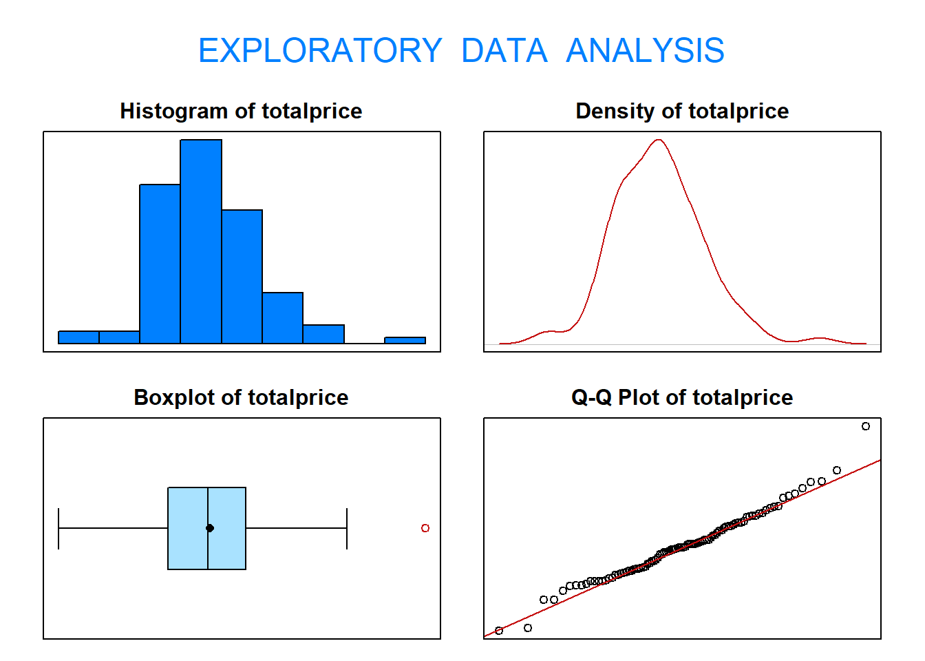
To solve this problem, start by selecting the data we are interested in and then verify the reasonableness of the normality assumption.
##     Size (n)      Missing      Minimum       1st Qu         Mean       Median
## 9.400000e+01 0.000000e+00 1.780000e+05 2.922500e+05 3.358840e+05 3.335000e+05
##       TrMean       3rd Qu          Max        Stdev          Var      SE Mean
## 3.347802e+05 3.730000e+05 5.600000e+05 6.183026e+04 3.822981e+09 6.377304e+03
##       I.Q.R.        Range     Kurtosis     Skewness     SW p-val
## 8.075000e+04 3.820000e+05 1.101000e+00 4.330000e-01 1.250000e-01
The results from applying eda(), suggest the appraised price for \(90m^2\) or larger pisos follows a normal distribution. Now, continue with the five-step procedure.
4.2 Step 1 - Hypotheses
Hypotheses — The null and alternative hypotheses to test whether the variability in price for \(90m^2\) or larger pisos is greater than \(60,000^2\text{€}^2\), are
\[H_0 : \sigma^2 = 60,000^2 \quad \text{versus} \quad H_1 : \sigma^2 > 60,000^2 \]
This is a one-tail test as as we want to know if the variability in price of pisos that are \(90m^2\) or larger is in fact \(60,000^2\text{€}^2\) or if it is greater than that. Two-tailed would test for any difference from \(60,000^2\text{€}^2\) not just greater than.
4.3 Step 2 - Choosing a Test Statistic
The test statistic chosen is \(S^2\) because \(E[S^2] = \sigma^2\).
## [1] 3822980710The value of this test statistic is \(s^2=3822980710\).
The standardised test statistic under the assumption that \(H_0\) is true and its approximate distribution are:
\[ \frac{(n-1)S^2}{\sigma^2_0}\quad \sim \quad \chi^2_{n-1},\] where \(n\) denotes the sample size and \(\sigma_0^2=60000^2\) in this case. This is what will be used to complete the test.
4.4 Step 3 - Hypothesis Test Calculations
4.4.1 Finding the rejection region
In this dataset, \(n = 94\) (which can be seen from Size (n) in the summary statistics above), so the standardised test statistic is distributed \(\chi^2_{93}\). Moreover, since \(H_1\) is an upper one-sided hypothesis, the rejection region is the \(\chi^2_{obs} > \chi^2_{0.95;93}\)
Using R code or the statistical tables, the \(t\)-value that corresponds to our significance level (critical value) is \(\chi^2_{0.95;93} = 116.511\).
## [1] 116.511This gives us the critical value and the significance level which make up the rejection region (what we will compare our result to). Remember sketching or graphing the \(\chi^2\) distribution and regions might help.
The rejection region is the area in which we would reject the null hypothesis. The critical value is the \(t\) value that corresponds to the significance level of 0.05, and hence is the bottom limit of our rejection region.
The probability of observing our test statistic (sample variance) or more extreme values under the null hypothesis is the \(p\)-value.
To reject a null hypothesis in this case we need the standardisd test statistic to be greater than the critical value and hence our \(p\)-value < 0.05.
4.4.2 Finding the standardised test statistic and \(p\)-value
The value of the standardised test statistic is given by \(\chi^2_{obs}\) = \(\frac{(n-1)s^2}{\sigma^2_0} = \frac{(94-1)*3822980710}{60,000^2} = 98.7603\).
## [1] 98.76034We should use R to find the corresponding \(p\)-value \(\mathrm{P}(\chi^2_{93} \geq 98.7603)\).
## [1] 0.3218218The \(p\)-value is equal to \(0.3218\) in this case.
You may want to sketch or plot this test graphically if you need help make a visual comparison between the value of test statistic and the rejection region we found above.
4.5 Step 4 - Statistical Conclusion
To draw our conclusions we need to consider our rejection region. Remember this is at the upper end of the \(\chi^2\)-distribution for this one-sided test.
QUESTION: Do we reject the null hypothesis?
I. From the rejection region, we fail to reject \(H_0\) because the standardised test statistic is less than the critical value and hence is not in the rejection region, i.e. \(\chi^2_{obs} = 98.7603 < 116.511\).
OR
- From the \(p\)-value, we fail to reject \(H_0\) because the \(p\)-value \(0.3218 > 0.05\).
Whichever method we use, we fail to reject \(H_0\).
4.6 Step 5 - English Conclusion
What does the previous statistical conclusion mean for the data and the purpose of the test?
Is there statistical evidence to suggest the variance for the appraised price of \(90m^2\) or larger pisos is greater than \(60,000^2\text{€}^2\)?
QUESTION: Which of the following is the correct conclusion of our test?