4 Example 2: Simulating random variables

We can use R to generate random variables. Here we will generate two random variables, \(X\) and \(Y\), that are, or aren't, related to each other in some form. This can help us understand the relationship between two variables and how they may be correlated.

4.1 Independent random variables

Let's start by first generating two random variables that are independent of one another. You have already been introduced to the normal distribution, where some random variable, \(X\), is centred at mean \(\mu\), with variance \(\sigma^2\), such that \(X \sim N(\mu, \sigma^2)\).

To generate random variables from the normal distribution we can use the rnorm command. For example, let's say we want to generate \(n=30\) samples from two random variables, \(X\) and \(Y\), each with mean \(\mu = 10\), and standard deviation \(\sigma = 1\), we can do this as follows:

n <- 30
mu <- 10
sigma <- 1
set.seed(1)
y <- rnorm(n, mean = mu, sd = sigma)
x <- rnorm(n, mean = mu, sd = sigma)

Note: since we are generating random numbers it is best to use the command set.seed beforehand to be able to replicate the results. For example, if we first run the line set.seed(1), and then the above code, we will generate the same random variables x and y, and a different set if we change the seed value.

This gives us our random variables \(X\) and \(Y\), generated independently of one another, and so we should expect to see no relationship between them. Using set.seed(1) to obtain \(X\) and \(Y\), a scatterplot of their relationship is shown in Figure 4.1.

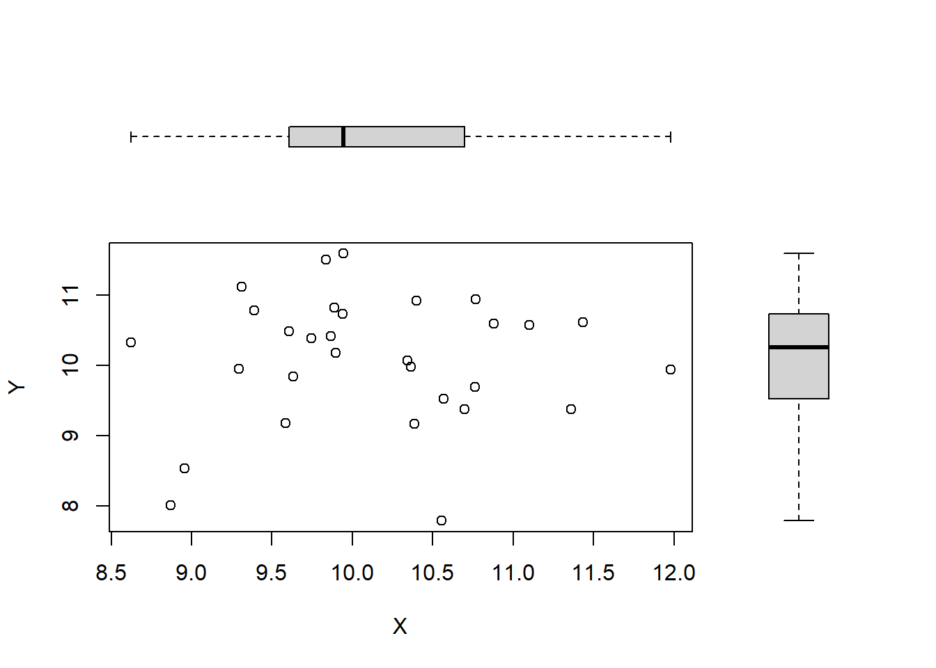
Figure 4.1: Scatterplots of independent random variables.

QUESTION: What can we say about the relationship between \(X\) and \(Y\) from Figure 4.1? What can be said about the two boxplots in Figure 4.1?

QUESTION: Use R as a calculator or the cor() function to calculate the correlation between the two variables. What does this value tell us about the their relationship?

The sample correlation \(r\) = , suggesting a strongmoderateweakno linear relationship between \(X\) and \(Y\).

x_mean <- mean(x)
y_mean <- mean(y)
r <- sum((x-x_mean) * (y-y_mean)) / sqrt(sum((x-x_mean)^2)*sum((y-y_mean)^2))
print(r)

## [1] 0.04866964

cor(x,y)

## [1] 0.04866964

4.2 Correlated random variables

Let us now look at how to generate random variables that are correlated in some way. To do that we will need to obtain the covariance or correlation matrix, and generate the random variables from a multivariate normal distribution. The multivariate normal distribution is a generalisation of the normal distribution to higher dimensions, and as multivariate data analysis is not covered until Honours level we will simplify things a little.

To generate correlated random variables we can use the mvrnorm command (load library(MASS)). This requires us to obtain the covariance matrix, \(\Sigma\), explaining the relationship between our two random variables. As you will find out in 2X, the covariance is scale dependent, and as such, the correlation is often easier to use and interpret.

We simplify things by generating random variables, \(X\) and \(Y\), such that their variances are the same and equal to one. Assuming \(\text{Var}(X) = \text{Var}(Y) = 1\), we can then see from formula (1.1) that

\[\rho(X,Y) =\frac{\mathrm{Cov}(X,Y)}{\sqrt{\mathrm{Var}(X)\mathrm{Var}(Y)}} = \frac{\mathrm{Cov}(X,Y)}{\sqrt{1 \cdot 1}} = \mathrm{Cov}(X,Y),\]

that is, the correlation and covariance are the same. This now means that the covariance matrix, \(\Sigma\), and the correlation matrix, \(P\), are now equivalent, such that,

\[\Sigma = \begin{bmatrix} \text{Var}(X) & \text{Cov}(X, Y) \\ \text{Cov}(X, Y) & \text{Var}(Y) \end{bmatrix} = \begin{bmatrix} 1 & \rho(X, Y) \\ \rho(X, Y) & 1 \end{bmatrix} = P.\]

Now, let's say we want to generate two random variables, \(X\) and \(Y\), from a multivariate normal distribution, such that \((X, Y) \sim N(\boldsymbol{\mu}, \Sigma)\). This can be done using the mvrnorm command as follows:

library(MASS)
set.seed(1)
n <- 30
mu <- c(10, 10)
rho <- 0.85
Sigma <- matrix(rho, nrow = 2, ncol = 2) + diag(2) * (1 - rho)
rand.vars <- mvrnorm(n, mu = mu, Sigma = Sigma)
x <- rand.vars[, 1]
y <- rand.vars[, 2]

Here we have generated \(n = 30\) random samples from a multivariate normal distribution for \(X\) and \(Y\), with mean vector \(\boldsymbol{\mu}^\top =\begin{bmatrix} \mu_X & \mu_Y \end{bmatrix} = \begin{bmatrix}10 & 10 \end{bmatrix}\), and correlation matrix, \(P\), such that \(\rho(X, Y) = 0.85\).

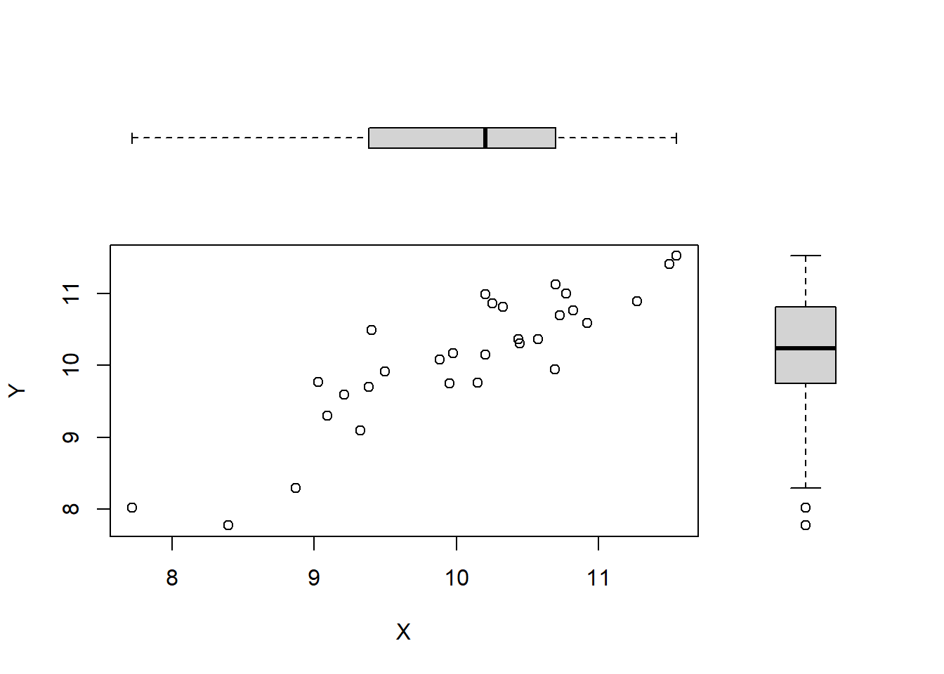
Figure 4.2: Scatterplots of correlated random variables.

QUESTION:

1. What can we say about the relationship between \(X\) and \(Y\) from the scatterplot in Figure 4.2?

2. Calculate the sample correlation coefficient, \(r\). Is this the same as the correlation parameter, \(\rho\), used to generate the data?

The sample correlation coefficient will not be exactly the same as the correlation parameter since the simulated data are random samples from the true population.

3. What happens with the sample correlation, \(r\), and the 'true' correlation, \(\rho\), as the number of samples, \(n\), increases?

4. Edit the R code to obtain a weak-to-moderate positive linear relationship between \(X\) and \(Y\). Use a scatterplot to examine this relationship, and use the cor command to see if the sample correlation matches that used to simulate the data.

5. Generate two random variables that exhibit a moderate-to-strong negative linear relationship. Use a plot to display this relationship, and obtain an estimate of the sample correlation coefficient.