3 Example 1: The 5 Steps of Hypothesis Testing

An experiment was conducted to investigate how the resistance of rubber to abrasion is affected by the hardness of the rubber and its tensile strength. The data come from Hand et al. (1994, Data Set #6, Abrasion Loss) and are stored in the data frame Rubber of the MASS package. The abrasion loss is measured in grams/hour; the hardness, in degrees shore; and the tensile strength, in \(kg/cm^2\). Use the five-step procedure to test whether \(\mu < 170\) for abrasion loss (loss) with 95% confidence.

To open this data file, type:

library(MASS)
RUBBER<- Rubber

This will assign the data to the object RUBBER. To view the data, type

RUBBER

into the script file and running that line by either placing the cursor on the line and pressing Ctrl and Enter, or by clicking on the Run button in the top-right corner of the script file. The data will then appear in the Console window below.

A spreadsheet of the data can be viewed by typing:

fix(RUBBER)

but note that you will need to close this window before trying to excute any further commands. The spreadsheet can also be viewed by clicking on the RUBBER object in the Environment (top right of the screen).

3.1 Verifying normality

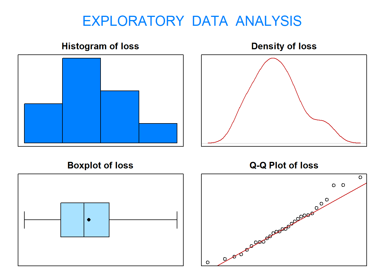
To solve this problem, start by verifying the normality assumption of the data using exploratory data analysis (EDA()).

library(PASWR)
with(data = RUBBER, EDA(loss))

## Size (n)  Missing  Minimum   1st Qu     Mean   Median   TrMean   3rd Qu 
##   30.000    0.000   32.000  113.250  175.433  165.000  173.536  220.500 
##      Max    Stdev      Var  SE Mean   I.Q.R.    Range Kurtosis Skewness 
##  372.000   88.085 7759.013   16.082  107.250  340.000   -0.522    0.433 
## SW p-val 
##    0.505

Based on the graphical output from the function eda(), it is not unreasonable to assume that abrasion loss follows a normal distribution. Now, proceed with the five-step procedure.

3.2 Step 1 - Hypotheses

To test if mean abrasion loss is less than \(170\), the hypotheses are:

\[H_0 : \mu = 170 \quad \text{verses} \quad H_1 : \mu < 170\]

This is a one-tail test as as we want to know how different the loss is from a mean of 170 (specifically less than) rather than just if it is different which would give the two-tail hypotheses \(H_0 : \mu = 170\) versus \(H_1 : \mu \neq 170\).

3.3 Step 2 - Choosing a Test Statistic

The test statistic chosen is \(\bar{X}\) because \(E[\bar{X}] = \mu\).

xbar <- mean(RUBBER$loss)
xbar

## [1] 175.4333

The value of this test statistic is \(\bar{x} = \frac{\sum^n_{i=1}x_i}{n} = 175.4333\)

We have this as our test statistic because we want to evaluate the mean value.

We will determine the probability of obtaining that test statistic (sample mean) when the null hypothesis is true. We do this with standardisation and the probability is called the \(p\)-value which we will find soon.

The standardised test statistic under the assumption that \(H_0\) is true is distributed \(\frac{\bar{X}−\mu_0}{S/\sqrt{n}} \sim t_{30-1}\).

3.4 Step 3 - Hypothesis Test Calculations

3.4.1 Finding the Rejection Region

Because the standardised test statistic is distributed \(t_{29}\) and \(H_1\) is a lower one-sided hypothesis, the rejection region is the \(t_{obs} \leq t_{0.05; 29}\).

From the statistical tables, the \(t\)-value that corresponds to our significance level (critical value) is \(t_{0.05; 29} = −1.6991\). Remember this is negative because we are discussing the lower tail of the \(t\)-distribution.

This same \(t\)-value can be found using R:

RR <- qt(0.05, df = 29)
RR

## [1] -1.699127

Graphically the rejection region is as follows:

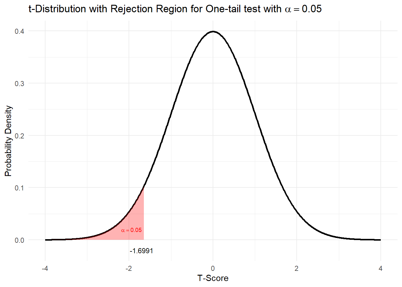
The rejection region is the area in which we would reject our null hypothesis. The critical value is the \(t\)-value that corresponds to \(p=0.05\), and hence is the top limit of our rejection region.

The probability of observing our test statistic (sample mean) or more extreme values under the null hypothesis is the \(p\)-value.

To reject the null hypothesis in this case we need our standardisd test statistic to be less than our critical value and hence our \(p\)-value < 0.05

3.4.2 Finding the standardised test statistic and \(p\)-value

The value of the standardised test statistic is given by \(\frac{\bar{X}−\mu_0}{S/\sqrt{n}} = \frac{175.4333−170}{S/\sqrt{n}}\). We can obtain \(S\) and \(n\) in R by using:

S <- sd(RUBBER$loss)
S

## [1] 88.08526

n <- length(RUBBER$loss)
n

## [1] 30

This gives our standardised test statistic \(t_{obs}=\frac{\bar{X}−\mu_0}{S/\sqrt{n}} = 0.3378\):

sta.test.stat <- (175.4333-170)/(S/sqrt(n))
sta.test.stat

## [1] 0.3378478

The \(p\)-value that corresponds to our standardised test statistic, \(P(t_{29} \leq 0.3378)\) is:

pvalue <- pt(0.3378478, df=29)
pvalue

## [1] 0.6310443

The standardised test statistic can be found using:

Test <- t.test(RUBBER$loss, mu = 170, alternative = "less")
Test

## 
##  One Sample t-test
## 
## data:  RUBBER$loss
## t = 0.33785, df = 29, p-value = 0.631
## alternative hypothesis: true mean is less than 170
## 95 percent confidence interval:
##      -Inf 202.7589
## sample estimates:
## mean of x 
##  175.4333

Graphically this could be shown:

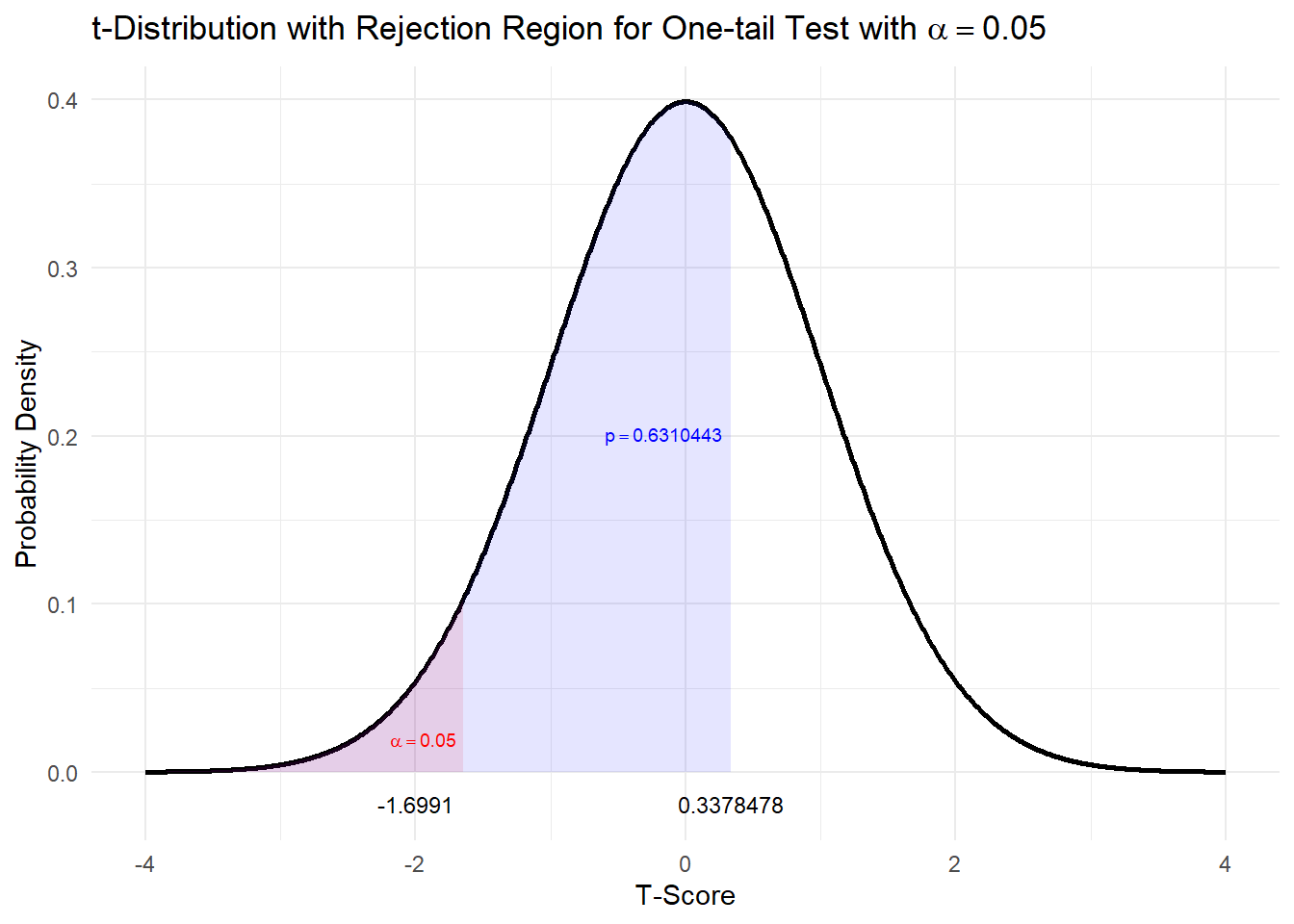
Our standardised test statistic is greater than the critical value and outside the rejection region. The \(p\)-value is greater than \(\alpha\).

3.5 Step 4 - Statistical Conclusion

To draw conclusions we need to consider the rejection region:

Is the value of standardised test statistic inside the rejection region? Is the \(p\)-value smaller than 0.05?

QUESTION: Do we reject the null hypothesis?

I. From the rejection region, we fail to reject \(H_0\) because the standardised test statistic is greater than the critical value and hence outside the rejection region i.e. \(t_{obs} = 0.3378 > -1.6991\).

From the \(p\)-value, we fail to reject \(H_0\) because the \(p\)-value is \(0.631 > 0.05\).

Whichever method we use, we fail to reject \(H_0\).

3.6 Step 5 - English Conclusion

What does the above statistical conclusion mean for the data and the purpose of the test?

Is there statistical evidence to suggest a mean less than 170?

QUESTION: Which of the following is the correct conclusion of our test?

There is sufficient evidence to suggest the mean abrasion loss is less than 170. We cannot conclude if there is sufficient evidence to suggest the mean abrasion loss is less than 170. There is not sufficient evidence to suggest the mean abrasion loss is less than 170. There is sufficient evidence to suggest the mean abrasion loss is greater than 170.