4 Example 2: Power of a test
A cell phone provider has estimated that it needs revenues of €2 million per day in order to make a profit and remain in the market. If revenues are less than €2 million per day, the company will go bankrupt. Likewise, revenues greater than €2 million per day cannot be handled without increasing staff. Assume that revenues follow a normal distribution with \(\sigma =\) €0.5 million and a mean of \(\mu\).
To find out more about their revenue they want to perform a hypothesis test \(H_0 : \mu = 2\) versus \(H_1 : \mu \neq 2\). To understand more about how hypothesis tests work, three scenarios will be presented to show how the power of a test can change: varying \(\mu\), varying significance level and varying sample size.
The power function is:
\[\text{Power}(\theta) = P(\text{reject }H_0|H_0 \text{ is false}) = P(\text{accept }H_1|H_1) = 1-\beta(\theta)\]
where \(\beta(\theta)\) is the probability of a type II error at a given \(\theta\).
4.1 Question 1
Graphically depict the power function for testing \(H_0 : \mu = 2\) versus \(H_1 : \mu \neq 2\) if \(n = 150\) and \(\alpha = 0.05\) for values of \(\mu\) ranging from 1.8 to 2.2.
First, think about whether we are doing a one or two-tailed test and what values represent rejecting or no-rejecting the null hypothesis.
Next, create a vector of the values of \(\mu\).
Subsequently, find the critical values for the chosen significance level \(\alpha\), which will be used to calculate the power for each \(\mu\).
The power values could be saved into a data frame to make the plotting easier.
mu <- seq(from = 1.8, to = 2.2, length = 500)
n <- 150
alpha <- 0.05
sigma <- 0.5

lcv <- qnorm(alpha/2, 2, sigma/sqrt(n))
ucv <- qnorm(1 - alpha/2, 2, sigma/sqrt(n))

Power <- pnorm(lcv, mu, sigma/sqrt(n)) + pnorm(ucv, mu, sigma/sqrt(n), lower = FALSE)

DF <- data.frame(mu, Power)
Once we have values for how the power function changes with \(\mu\), we could use ggplot to create the graph:
ggplot(data = DF, aes(x = mu, y = Power)) +
  geom_line(color = "red") +
  theme_bw() +
  labs(x = expression(mu), y = expression(Power~(mu))) +
  geom_hline(yintercept = 0.05, color = "blue", lty = "dashed")
4.2 Question 2
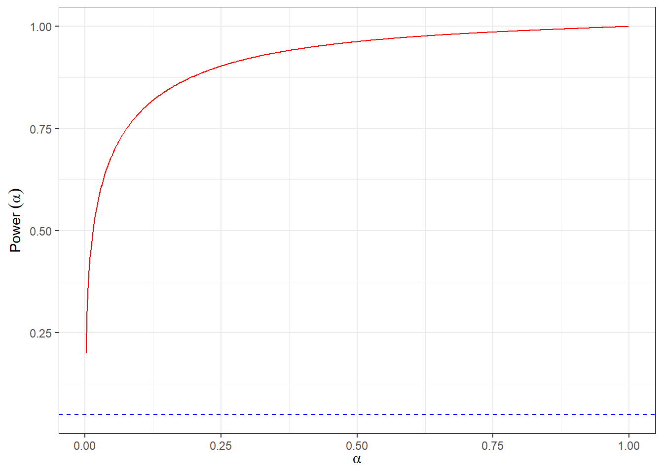
Graphically depict the power function for testing \(H_0 : \mu = 2\) versus \(H_1 : \mu \neq 2\) when \(\mu_1 = 2.1\) and \(n = 150\) for values of \(\alpha\) ranging from 0.001 to 0.999.
Think about whether you are doing a one or two-tailed test and what values represent rejecting or no-rejecting the null hypothesis.
First create a vector of values of \(\alpha\).
Then you will need to find the critical values for each \(\alpha\) which will be used to calculate the corresponding test powers.
The power values could be saved into a data frame to make the plotting easier.
4.3 Question 3
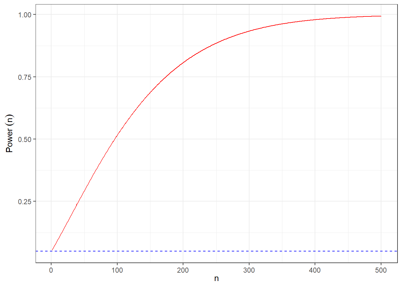
Graphically depict the power for testing \(H_0 : \mu = 2\) versus \(H_1 : \mu \neq 2\) when \(\mu_1 = 2.1\) and \(\alpha = 0.05\) for values of \(n\) ranging from 1 to 500.
Create a vector of values of \(n\) and then find the critical values for each \(n\) which will be used to calculate the corresponding test powers.