2 Example 1: Crime

We briefly looked at this data in the lectures. Here 50 US states were investigated in terms of their crime rates (per 100,000 people), which includes crimes such as murder, assault, and car theft. Some demographic information about each state was also recorded, such as the number of police and prisoners per 100,000 people, the percentage of population living in poverty, and the percentage of high school dropouts (i.e. 16-19 year olds who were not in school and did not finish the 12\(^\text{th}\) grade). The question of interest is whether we can predict US crime rates from the high school dropout rates and other predictors?

The data are available from the csv file crime.csv and contain six columns, described as follows:

C1	C1.T	US state
C2	Crime	Crime rate per 100,000
C3	Police	Number of police per 100,000
C4	Prison	Number of prisoners per 100,000
C5	Poverty	Percentage of population living in poverty
C6	Dropout	Percentage of high school dropouts

2.1 Simple linear regression

TASK 1

1. Use plot or pairs to visualise the data and determine which predictors may be useful in predicting Crime.

The R command pairs() may be used to see the relationships between all variables.

crime <- read.csv("crime.csv")
pairs(crime[,-1], lower.panel = NULL) # We add [,-1] to the end of crime to remove the first column which has non-numeric arguments (state names)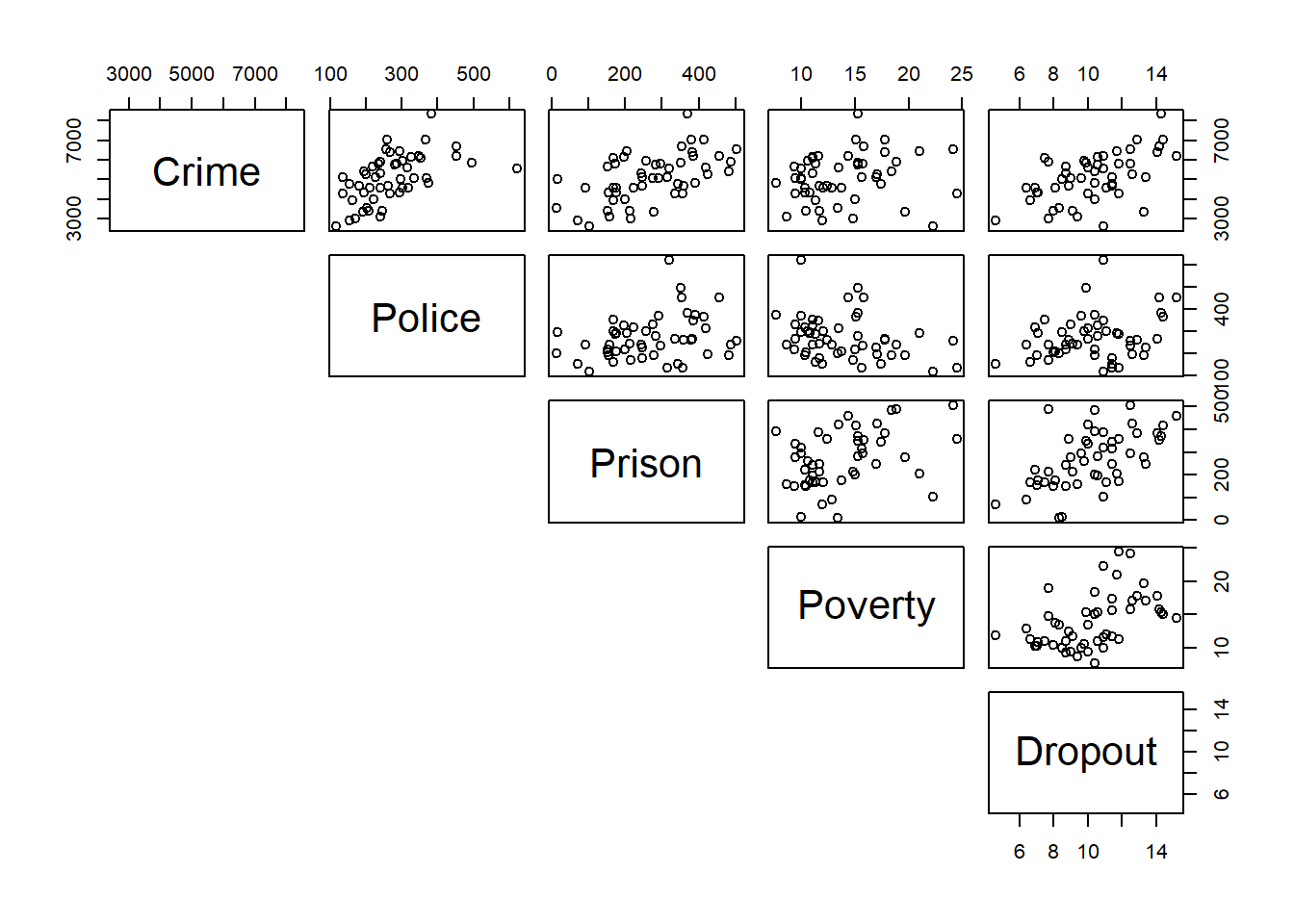

Apart from Dropout which has been discussed in the lectures, there may also be a positive linear relationship between Crime and Police and between Crime and Prison, though the relationship doesn't seem to be very strong.

2. Build a simple linear regression model with Dropout as the predictor and interpret estimated coefficients.

According to the model, when Dropout is equal to 0, the crime rate would be roughly . For every 1% increase in the % of high school dropouts, the expected crime rate (per 100,000) would increasedecrease by .

Use lm to build a linear regression model and summary() to find the coefficients.

3. The formula for the least squares estimates for the model parameters is

\[\hat{\boldsymbol \beta} = \begin{bmatrix} \hat{\beta_0} \\[0.5em] \hat{\beta_1} \end{bmatrix} = \begin{bmatrix} \overline{Y} - \hat{\beta_1} \overline{x} \\[0.5em] \frac{\sum_i(x_i-\bar{x})(y_i-\bar{y})}{\sum_i(x_i-\bar{x})^2} \end{bmatrix}.\]

Use this formula to compute the least squares estimates for the model parameters, \(\overline{\beta_0}\) and \(\overline{\beta_1}\).

\(\hat{\beta}_0\) = , \(\hat{\beta}_1\) =

x<-crime$Dropout
y<-crime$Crime
x_mean <- mean(x)
y_mean <- mean(y)
S_xx <- sum((x-x_mean)^2)
S_xy <- sum((x-x_mean)*(y-y_mean))

2.1.1 Least squares estimates of model parameters in matrix notation

To use the formula for least squares estimation in matrix notation given by (1.2), we first need to find the design matrix, \(\mathbf{X}\). This can be done using the following R command:

X <- model.matrix(~Dropout, data = crime)

This gives us the design matrix, \(\mathbf{X}\), for the simple linear regression model in (1.1), where we have \(n = 50\) rows corresponding to each of the 50 US states, and \(p = 2\) columns corresponding to the model parameters \(\beta_0\) and \(\beta_1\). More generally this is written as \[\mathbf{X} =\begin{bmatrix} 1 & x_1 \\1 & x_2 \\ \vdots & \vdots \\ 1 & x_n\end{bmatrix} \] The first column of \(\mathbf{X}\) contains 1's as that is the column that multiplies the first component of the parameter vector \(\boldsymbol\beta = \begin{bmatrix} \beta_0 & \beta_1 \end{bmatrix}'\), and as can be seen from the model, the intercept term, \(\beta_0\), is constant across all \(i\) observations. The slope parameter, \(\beta_1\), is also constant, however, the differences in crime rates between states comes from changes in the percentage of high school dropouts, given by \(x_i\), which multiplies \(\beta_1\). The random errors, \(\epsilon_i\), also differ per state.

Next we need the following commands to calculate each component in the matrix formula of least squares estimation:

t       # gets the transpose of a vector or matrix
%*%     # multiplies matrices together
solve   # computes the inverse of a matrix

Let's compute \(\mathbf{X}'\mathbf{X}\) using the following R code:

XtX <- t(X) %*% X

This gives

\[\mathbf{X}'\mathbf{X} = \begin{bmatrix} 50.0 & 512.6 \\ 512.6 & 5538.8 \end{bmatrix}\]

Recall, if

\[\mathbf{A} = \begin{bmatrix} a & b \\ c & d \end{bmatrix} \quad\quad \text{then} \quad\quad \mathbf{A}^{-1} = \frac{1}{\text{det}\left(\mathbf{A}\right)}\begin{bmatrix} d & -b \\ -c & a \end{bmatrix} = \frac{1}{ad - bc}\begin{bmatrix} d & -b \\ -c & a \end{bmatrix}.\]

Given \(\mathbf{X}'\mathbf{X}\) above, compute its inverse \(\left(\mathbf{X}'\mathbf{X}\right)^{-1}\):

\[(\mathbf{X}'\mathbf{X})^{-1} = \hspace{9em}\]

To find \(\hat{\boldsymbol\beta}\) we also need to find \(\mathbf{X}'\mathbf{Y}\). Using the above commands, or by hand, compute \(\mathbf{X}'\mathbf{Y}\):

\[\mathbf{X}'\mathbf{Y} = \begin{bmatrix} & & & & \\\\ \\ \end{bmatrix}\]

Multiplying \(\left(\mathbf{X}'\mathbf{X}\right)^{-1}\) and \(\mathbf{X}'\mathbf{Y}\) then gives us the least squares estimates of the model parameters. By hand, compute the parameter estimates, \(\hat{\boldsymbol\beta}\), such that

\[\hat{\boldsymbol{\beta}} = (\mathbf{X}'\mathbf{X})^{-1}\mathbf{X}'\mathbf{Y} = \]

4. Use the R commands given above to compute \(\left(\mathbf{X}'\mathbf{X}\right)^{-1}\) and \(\mathbf{X}'\mathbf{Y}\), and hence \(\hat{\boldsymbol\beta}\), and compare the output with your handwritten results.

XtX_inv <- solve(XtX)
Y <- crime$Crime
XtY <- t(X) %*% Y
beta.hat <- solve(XtX) %*% XtY

We can also obtain the vector of random errors, \(\boldsymbol \epsilon\), by taking the difference between the observed values, \(\mathbf{Y}\), and the fitted values, \(\hat{\mathbf{Y}} = \mathbf{X}\hat{\boldsymbol\beta}\), using the command:

residuals <- Y - X %*% param.ests

2.2 Multiple linear regression

5. Use one or more predictors alongside Dropout to build a multiple linear regression model for explaining Crime.

Use the graph found using the pairs() command in (a) to select predictors that appear suitable for describing Crime.

Recall that a multiple linear regression model can be constructed using

model <- lm(Crime ~ Dropout + Predictor1 + Predictor2 + ..., data = crime)

6. Calculate the least squares estimates of parameters in the new multiple linear regression model using the formula in matrix notation.

The same steps can be followed as in (d), but the design matrix X has to be updated accordingly. Say we want to add Police and Prison variables to our model. We would then use the following code.

X <- model.matrix(~ Dropout + Police + Prison, data = crime)
Y <- crime$Crime

XtX <- t(X) %*% X
XtY <- t(X) %*% Y

beta.hat <- solve(XtX) %*% XtY
beta.hat

##                    [,1]
## (Intercept) 1513.317509
## Dropout      148.343452
## Police         4.782505
## Prison         2.794514