3 Exercise 1: SLR with no intercept
Introducing the data: Hubble's Constant
Source: Hubble, E. (1929) A Relationship Between Distance and Radial Velocity among Extra-Galactic Nebulae, Proceedings of the National Academy of Science, 168.
Context: In 1929 Edwin Hubble investigated the relationship between distance and radial velocity of extragalactic nebulae (celestial objects). It was hoped that some knowledge of this relationship might give clues as to the way the universe was formed and what may happen later. His findings revolutionised astronomy and are the source of much research today on the ‘Big Bang’. Given here is the data that Hubble used for 24 nebulae. It is of interest to determine the effect of distance on velocity.
Data: hubble.csv
Columns:
Distance - (in Megaparsecs) from EarthVelocity - recession (in km/sec)Read in the data using:
3.1 Exploratory analysis
TASK 2
- Produce a scatterplot of the data with
Velocityon the y-axis.
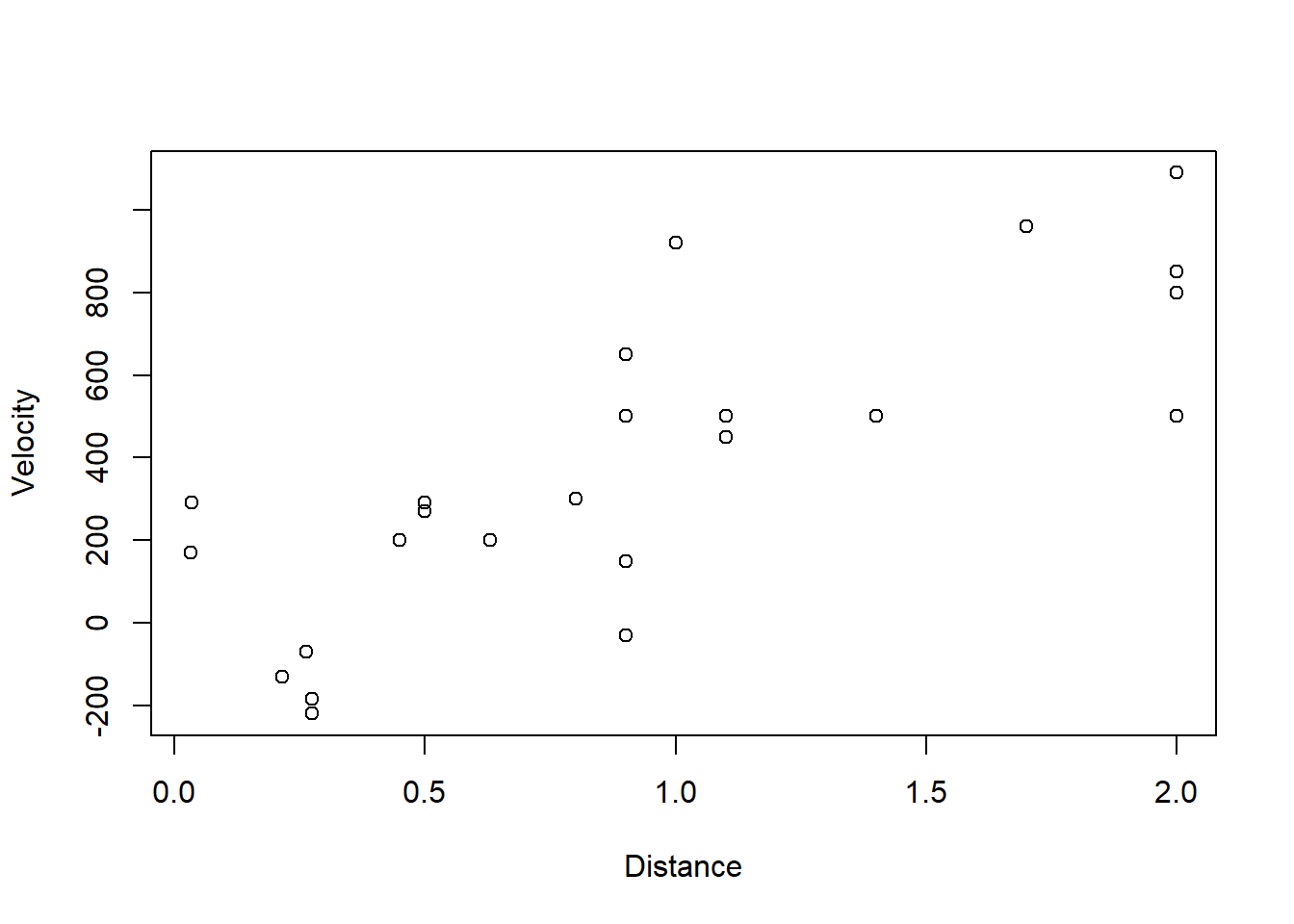
- Describe the shape of the relationship.
The relationship appears to be and it that the line passes through the origin.
3.2 Fitting a simple linear regression model
- Fit a simple linear regression model with the response variable
Velocityand the explanatory variableDistanceand write down the equation of the fitted line.
The equation of the fitted line is given by:
Velocity = + Distance
This is the line of best fit, describing the effect of distance on velocity.
- Produce a plot of the data including the fitted line.
A fitted line can be added to a plot using the command abline.
model_hubble <- lm(Velocity ~ Distance, data = hubble)
plot(Velocity ~ Distance, data = hubble)
abline(model_hubble)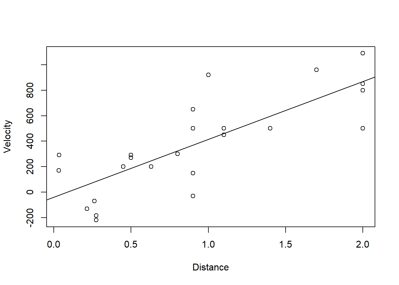
Now with OLS
- Fit a simple linear regression model with the response variable
Velocityand the explanatory variableDistanceand provide parameter estimates using the matrix formula of least squares estimation.
\(\hat{\boldsymbol{\beta}}=(\mathbf{X}'\mathbf{X})^{-1} \mathbf{X}'\mathbf{Y}\)
X <- model.matrix(~ Distance, data = hubble)
3.3 Fitting a linear model with no intercept
From the scatterplot in (a), it is plausible from the data that the regression line should be forced to go through the origin. A model with no intercept could be fitted using:
The inclusion of -1 is what removes the intercept term from the model fit.
Note down the equation of the fitted line that is given:
Velocity = Distance
If we save the model with and without intercept using
model.Int <- lm(Velocity ~ Distance, data = hubble)
model.NoInt <- lm(Velocity ~ -1 + Distance, data = hubble)
a plot of the data can be re-produced as before with the fitted lines from both linear models added using the command:
plot(Velocity ~ Distance, data = hubble)
abline(model.Int, col = "red")
abline(model.NoInt, col = "blue", lty = 2)
legend("topleft", legend = c("with intercept", "w/o intercept"), lty = c(1,2), col = c("red","blue"), bty = "n")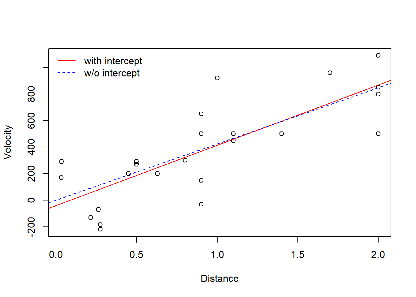
Figure 3.1: Scatterplot of Velocity versus Distance with two fitted models - simple linear regression model with and without the intercept.
The lty argument in abline changes the type/style of the line plotted, which is handy when printing in black and white.
A legend is also added to distinguish between the lines plotted.
Now with OLS
- Fit a simple linear regression model with the response variable
Velocityand the explanatory variableDistancebut with no intercept. Again use the matrix formula of least squares estimation.
X <- model.matrix(~ -1 + Distance, data = hubble)
DISCUSSION: Comparing the two fitted lines, is the model that passes through the origin plausible?