2 Example 1: Power transformation on \(Y\)

The stopping.csv file contains 63 observations of cars in the process of breaking. Our question of interest is: Can we determine if there is a relationship between the speed of cars and the distance taken to stop?

Data: stopping

Columns:

                      C1: Distance - stopping distance measured in feet

                      C2: Speed - Speed of the car as when it breaks in miles per hour

Read the data using

stopping <- read.csv("stopping.csv")

2.1 Exploratory analysis and model fitting

The scatterplot of distance (\(Y\)) against the speed (\(x\)) in Figure 2.1 (left) shows that the variables do not appear to be linearly related. The temptation in this case would be to apply a quadratic transformation for \(x\) give that the data are curved and concave. The centre plot in Figure 2.1 shows this transformation. It is linear, but the variance has a fanning effect. For this reason, we consider transforming \(Y\) using the square-root transformation (\(\sqrt{Y}\)), which should have a similar effect to our first attempt. The right plot in the figure now shows a linear relationship with constant variance between predictor and response.

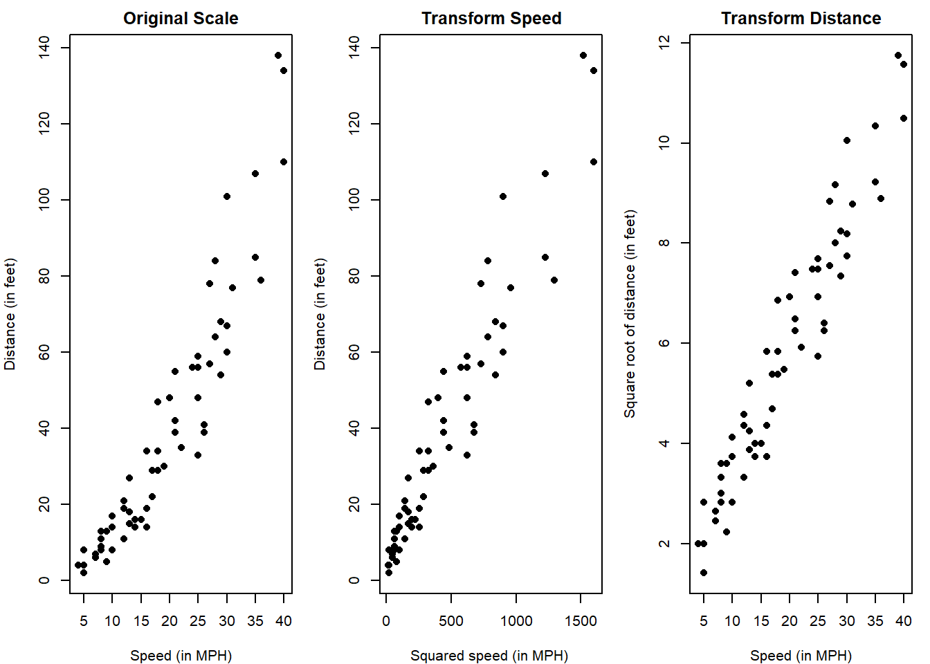
Figure 2.1: Left: scatterplot of Distance versus Speed. Centre: scatterplot of Distance versus square root of Speed. Right: scatterplot of square root of Distance versus Speed.

With a linear relationship, we can more appropriately use our simple linear regression model between \(\sqrt{\text{Distance}}\) (as new \(Y\)) and speed as \[Y_i = \beta_0 + \beta_1 x_i + \epsilon_i,\quad \epsilon_i \sim N(0,\sigma^2), \quad i = 1,\ldots, 63.\]

model.sqrt <- lm(I(Distance^0.5) ~ Speed, data = stopping)
# or 
# model.sqrt <- lm(sqrt(Distance) ~ Speed, data = stopping)

2.2 Assumption checking and interpretation

Figure 2.2 gives the residual plots after fitting a simple linear regression model to the original variables.

model.og <- lm(Distance ~ Speed, data = stopping)
plot(rstandard(model.og) ~ fitted(model.og), 
     pch = 16)
qqnorm(rstandard(model.og))
qqline(rstandard(model.og))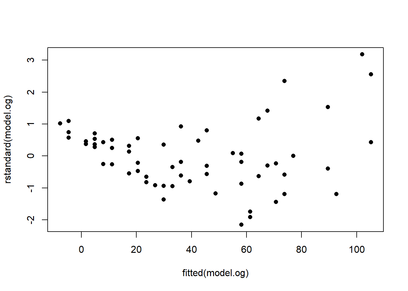

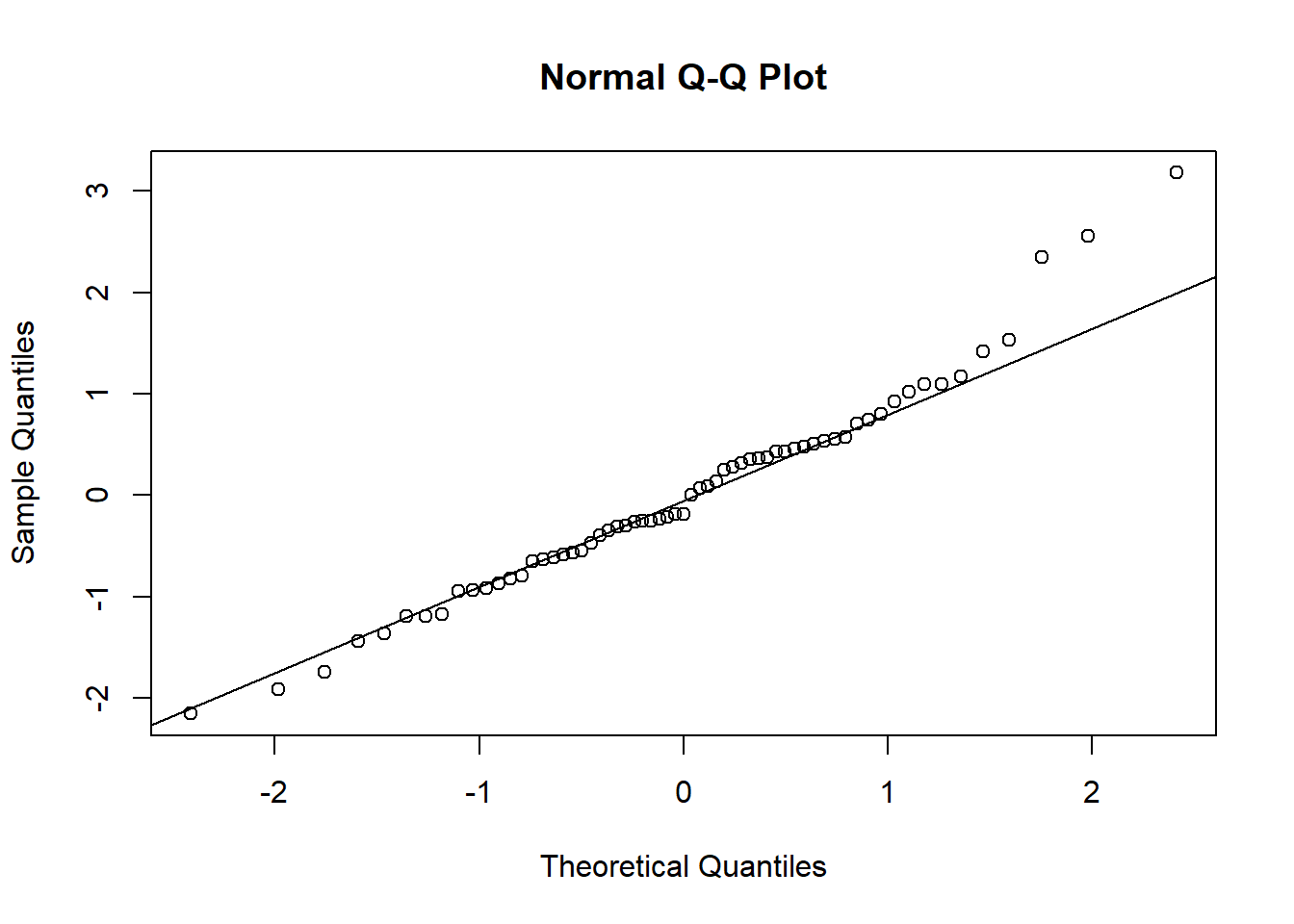
Figure 2.2: Residual plots from fitting a simple linear regression model to original variables. Top: Standardised residuals versus fitted values. Bottom: Normal probability (Q-Q) plot.

The plots show the problems of curvature, non-constant variance and non-normality, indicating that the wrong type of model was used.

Figure 2.3 gives the residual plots after fitting a simple linear regression model to the transformed variables.

model.sqrt <- lm(sqrt(Distance) ~ Speed, data = stopping)
plot(rstandard(model.sqrt) ~ fitted(model.sqrt), 
     pch = 16)
qqnorm(rstandard(model.sqrt))
qqline(rstandard(model.sqrt))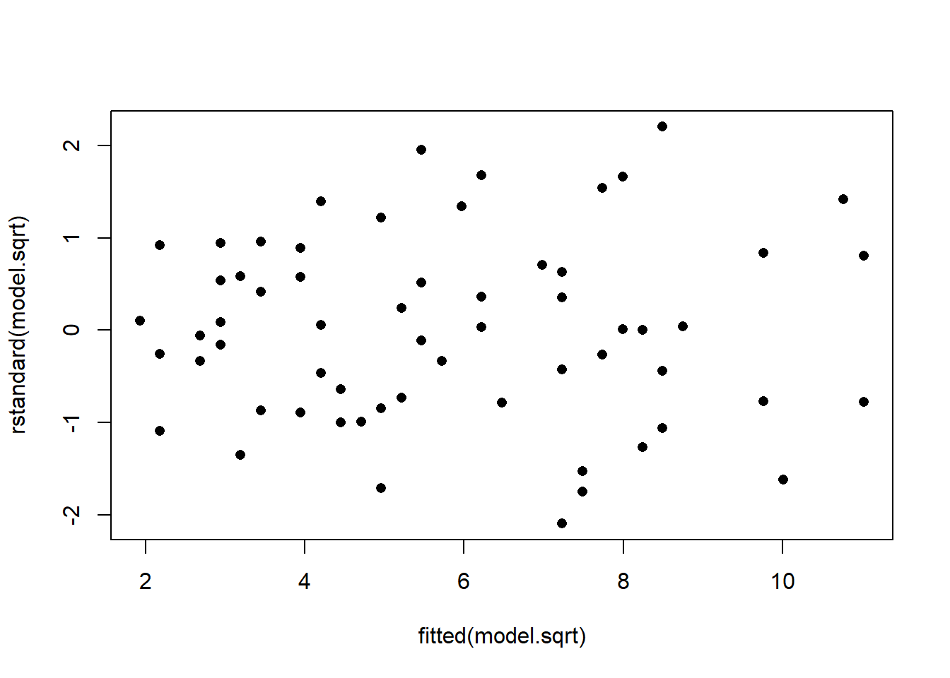

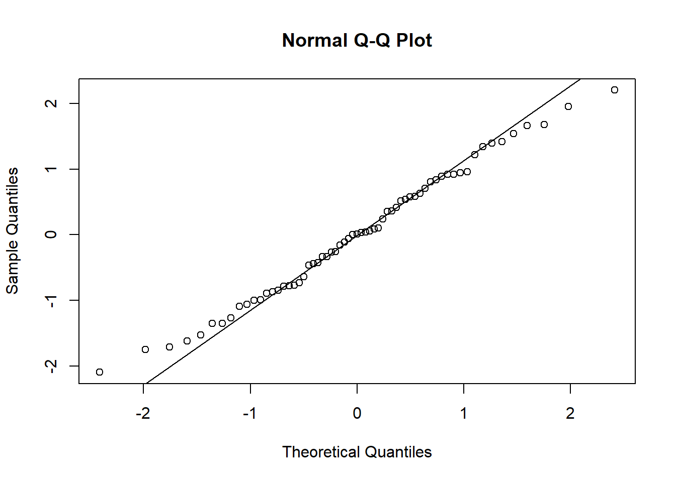
Figure 2.3: Residual plots from fitting a simple linear regression model to transformed variables. Top: Standardised residuals versus fitted values. Bottom: Normal probability (Q-Q) plot.

The curvature disappears and the variance is almost constant across the range of fitted values. The normality assumption, however, remains to be invalid. This is not ideal but, on the positive side, the estimates of parameters will not be affected and hence we can still use the model to describe the relationship between variables and make predictions.

summary(model.sqrt)

## 
## Call:
## lm(formula = sqrt(Distance) ~ Speed, data = stopping)
## 
## Residuals:
##     Min      1Q  Median      3Q     Max 
## -1.4879 -0.5487  0.0098  0.5291  1.5545 
## 
## Coefficients:
##             Estimate Std. Error t value Pr(>|t|)    
## (Intercept) 0.918283   0.197406   4.652 1.82e-05 ***
## Speed       0.252568   0.009246  27.317  < 2e-16 ***
## ---
## Signif. codes:  0 '***' 0.001 '**' 0.01 '*' 0.05 '.' 0.1 ' ' 1
## 
## Residual standard error: 0.7193 on 61 degrees of freedom
## Multiple R-squared:  0.9244, Adjusted R-squared:  0.9232 
## F-statistic: 746.2 on 1 and 61 DF,  p-value: < 2.2e-16

The interpretation of the parameters is always done in the scale of the model. For example, we have \(\beta_1 = 0.2526\), so we say that sqrt(Distance) changes \(0.2526\) feet for every \((mile/hour)\). If you are making predictions, you can back-transform the results to the original scale. You can do this by performing the inverse operation that you used for the transformation. If you used \(sqrt(Y)\) for the transformation, then the back-transformation requires you to square the data, \(\hat{Y}^2\), to put it back in the original scale.

Tasks

1. Write down the equation of the fitted model.

The regression equation is \[\sqrt{\text{Distance}} = 0.918 + 0.253 \cdot \text{Speed} \]

2. Based on the regression equation in (a), comment on the relationship between speed and square root of distance. In addition, pick a speed value yourself and predict the distance for this speed.

The estimated parameter of \(0.253\) suggests the square root of distance is positively linearly related to speed. As the speed increases by 1 MPH, the expected square root of distance increases by 0.253 feet.

When predicting the value of the response, we back transform the variable as \(\text{Distance} = (0.918 + 0.253 \cdot \text{Speed})^2\). For example, if the speed is 20 MPH, the predicted distance is \((0.918+0.252\cdot 20)^2 \approx 35.64\) feet.

Note that our model is built only for speed ranging from 4 to 40. It would be unwise to make predictions outside this range in the absence of other information.