4 Exercise 1: Identify the appropriate transformation

The following simulated data contain different non-linear relationships between response and predictor variables.

Data: SIMDATAXT and SIMDATAST

Columns:

                      C1: x1 - predictor 1

                      C2: x2 - predictor 2

                      C3: x3 - predictor 3

Read in the data using:

library(PASWR2)
data("SIMDATAXT")
data("SIMDATAST")

QUESTIONS:

1. Using the data SIMDATAXT, apply appropriate transformations to \(x_1\), \(x_2\), and \(x_3\) to linearise the relationships between the response and predictors one at a time.

It might be best if you break it down and address one predictor at the time.

Transform \(x_1\) You can begin by examining the relationship between \(y\) and \(x_1\) at the original scale and in a simple linear model.

# Plot relationship
plot(y ~ x1, data = SIMDATAXT)

# Fit and plot model
model1 <- lm(y ~ x1, data = SIMDATAXT)
plot(model1,which=c(1))

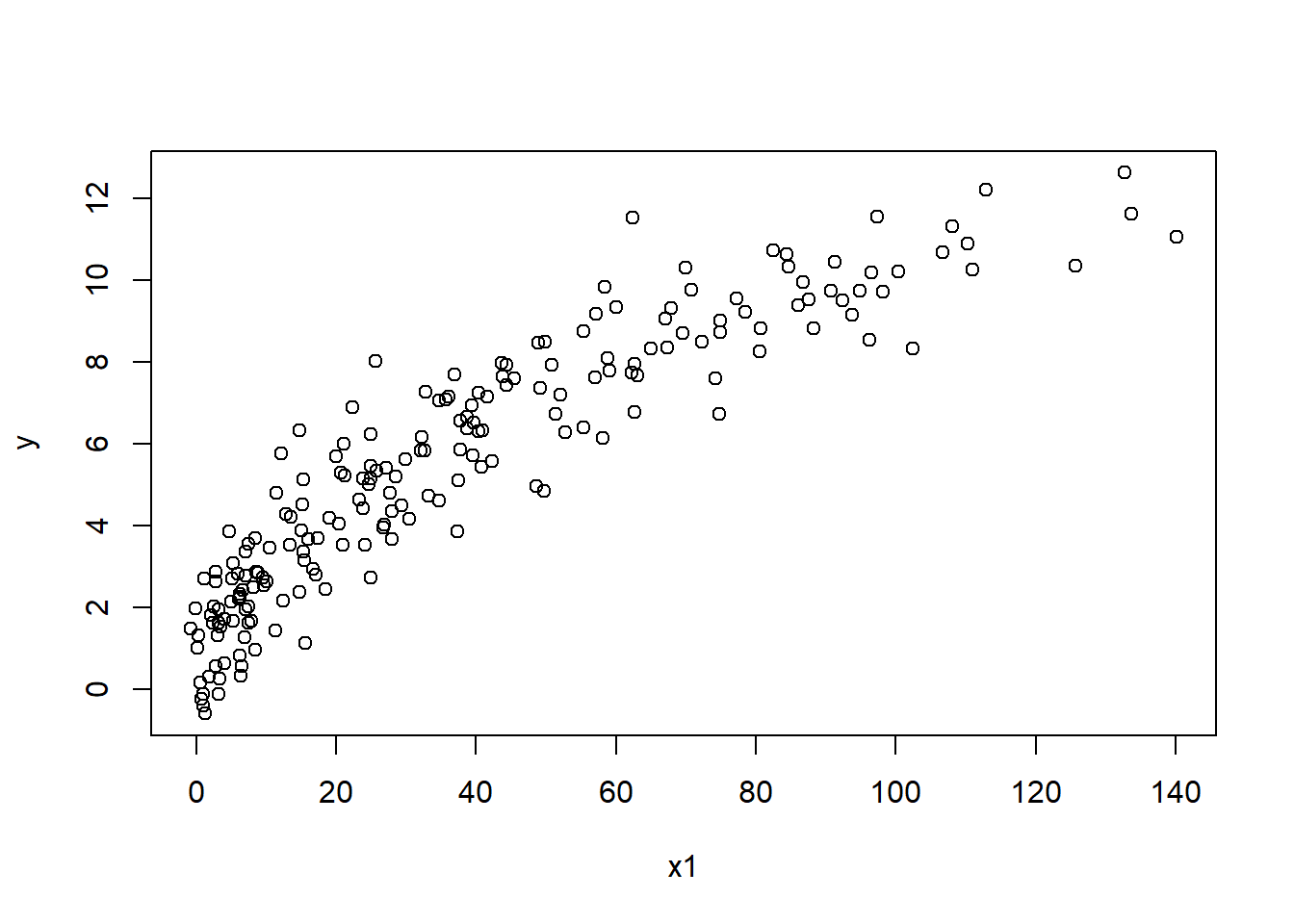
The relationship between \(y\) and \(x_1\) is curved and convex.

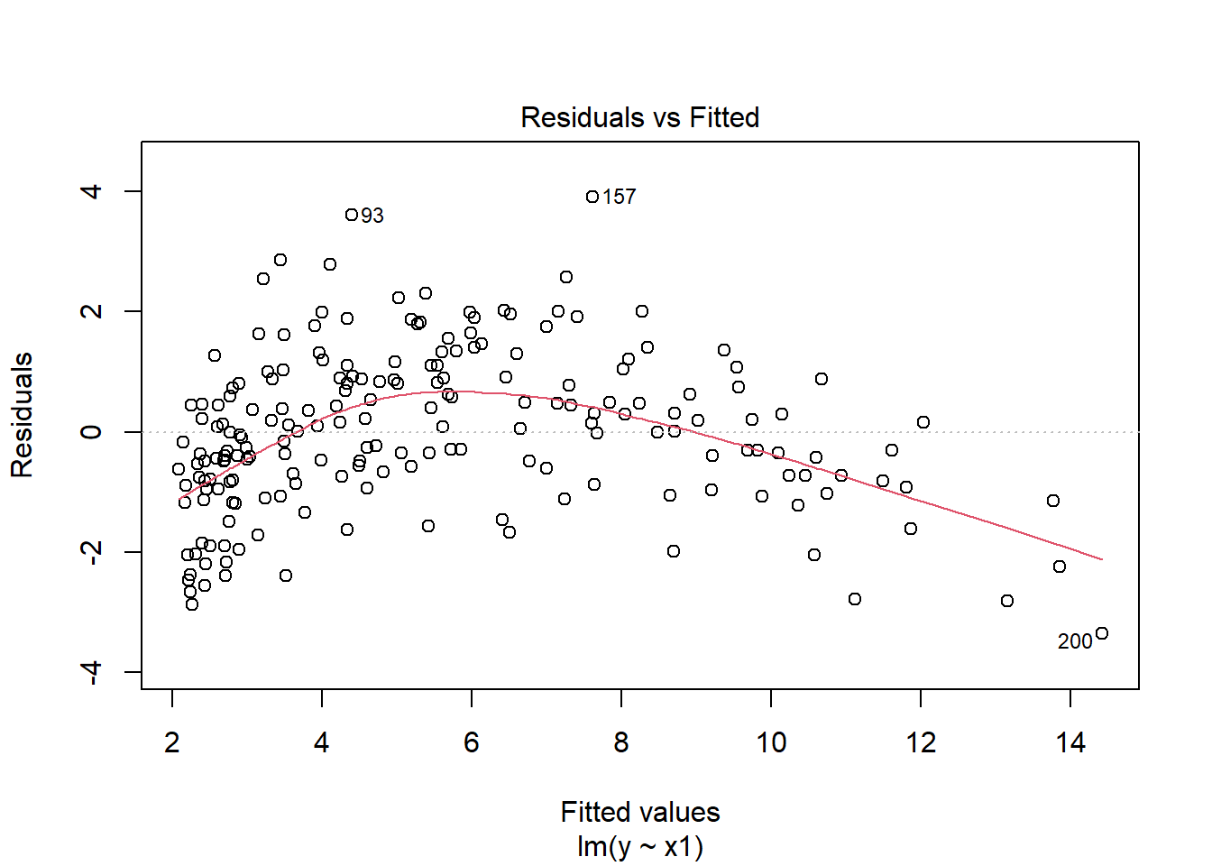
Apply the transformation you think is necessary and fit a model.

From the figures, the appropriate transformation of \(x_1\) is the square rootquadraticlogarithmicreciprocalnone .

# Before transformation
plot(y ~ x1, data = SIMDATAXT)
model1 <- lm(y ~ x1, data = SIMDATAXT)
plot(model1,which=c(1)
# Figures suggest a square root transformation
plot(y ~ sqrt(x1), data = SIMDATAXT)
model2 <- lm(y ~ sqrt(x1), data = SIMDATAXT)
plot(model2,which=c(1)) # Much better!

Transform \(x_2\) The second predictor can be evaluated in the same way as the first. You can begin by examining the relationship between \(y\) and \(x_2\) and the relationship between the two in a simple linear model using scatterplots.

# Plot relationship
plot(y ~ x2, data = SIMDATAXT)

# Fit and plot model
model3 <- lm(y ~ x2, data = SIMDATAXT)
plot(model3,which=c(1))

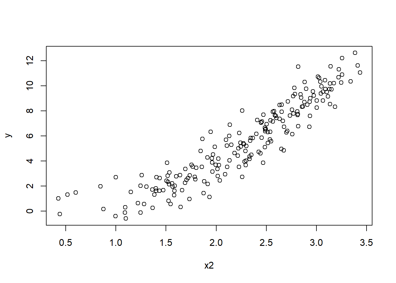
The relationship seems both curved and concave.

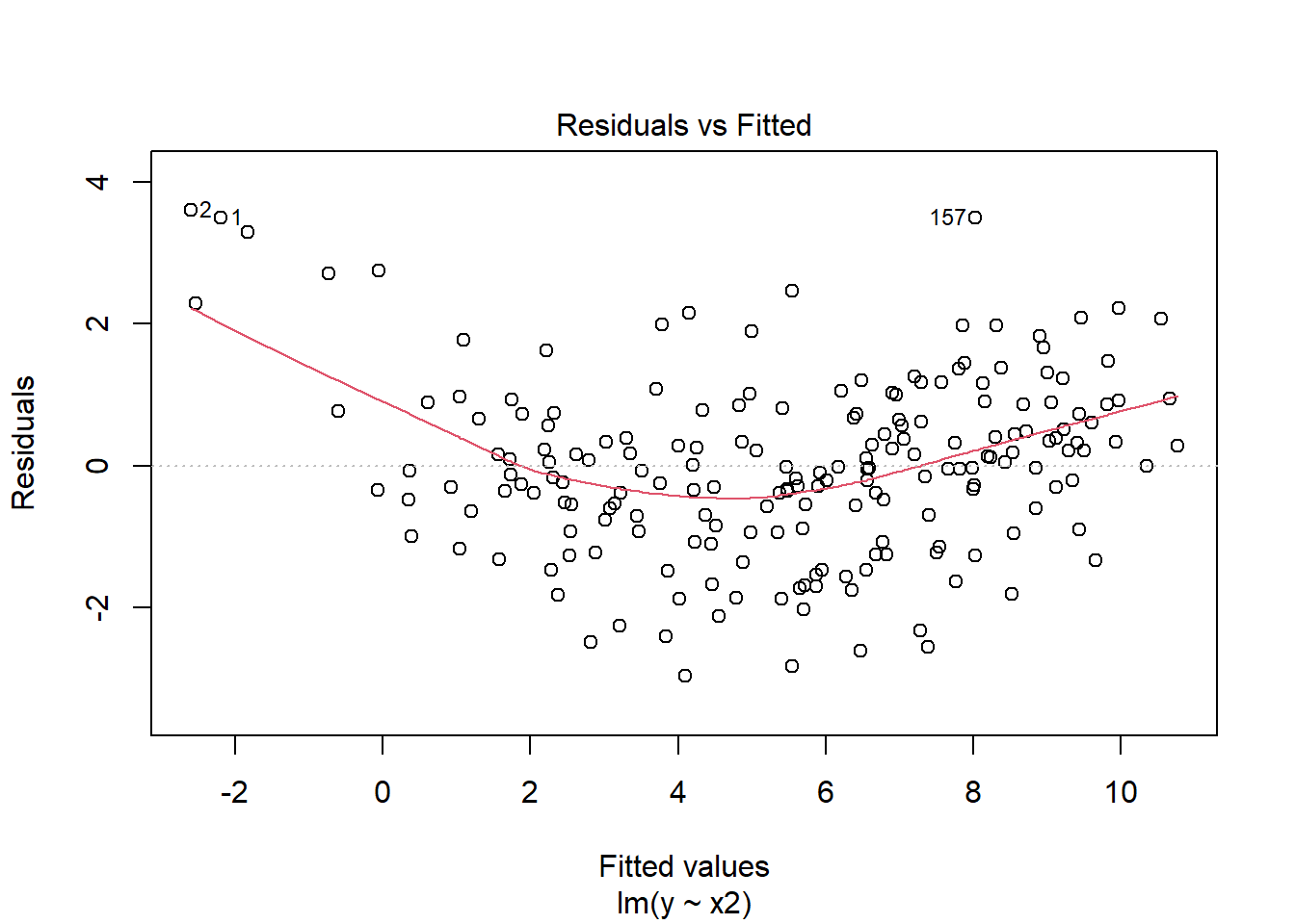
Apply the transformation you think is necessary and fit a model.

From the figures, the appropriate transformation of \(x_2\) is quadraticsquare rootlogarithmicreciprocalnone.

# Before transformation
plot(y ~ x2, data = SIMDATAXT)
model3 <- lm(y ~ x2, data = SIMDATAXT)
plot(model3,which=c(1))
# Figures suggest a square root transformation
plot(y ~ I(x2^2), data = SIMDATAXT)
model4 <- lm(y ~ I(x2^2), data = SIMDATAXT)
plot(model4,which=c(1)) 

Transform \(x_3\) Plot \(y\) and \(x_3\) and the residuals of a simple linear model to assess the relationship between the two.

# Plot relationship
plot(y ~ x3, data = SIMDATAXT)

# Fit and plot model
model5 <- lm(y ~ x3, data = SIMDATAXT)
plot(model5,which=c(1))

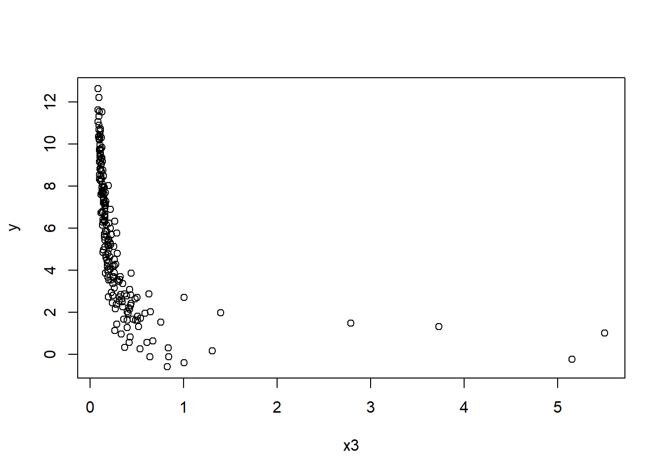
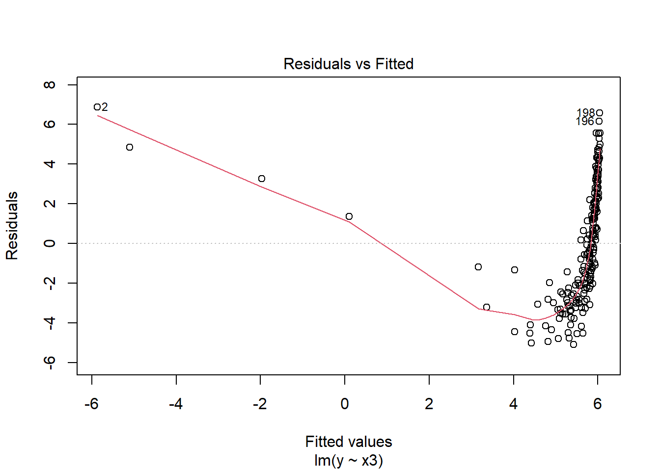
The relationship seems curved and concave.

Apply the transformation you think is necessary and fit a model.

The figures suggest a reciprocalsquare rootlogarithmicquadraticnone transformation for \(x_3\).

# Before transformation
plot(y ~ x3, data = SIMDATAXT)
model5 <- lm(y ~ x3, data = SIMDATAXT)
plot(model5)
# Figures suggest a square root transformation
plot(y ~ I(x3^(-1)), data = SIMDATAXT)
model6 <- lm(y ~ I(x2^(-1)), data = SIMDATAXT)
plot(model6) 

2. Using the data SIMDATAST, figure out the appropriate transformation for \(x_1\) and/or \(y\). Follow the usual steps by producing a scatterplot of \(y\) and \(x_1\) and the residuals of the simple linear model at original scale. Consider the possible transformations.

The figures suggest using a logarithmicsquare rootreciprocalquadraticnone transformation for Yx1bothnone.

# Before transformation
plot(y ~ x1, data = SIMDATAST)
model1b <- lm(y ~ x1, data = SIMDATAST)
plot(model1b)
# Figures suggest transforming the response
plot(log(y) ~ x1, data = SIMDATAST)
model2b <- lm(log(y) ~ x1, data = SIMDATAST)
plot(model2b) 

3. Using the data SIMDATAST, figure out the appropriate transformation for \(x_2\) and/or \(y\). Follow the steps outlined in (b).

The figures suggest using a reciprocalsquare rootlogarithmicquadraticnone transformation for Yx2bothnone.

# Before transformation
plot(y ~ x2, data = SIMDATAST)
model1c <- lm(y ~ x2, data = SIMDATAST)
plot(model1c)
# Figures suggest transforming the response
plot(log(y) ~ x2, data = SIMDATAST)
model2c <- lm(log(y) ~ x2, data = SIMDATAST)
plot(model2c)