5 Exercise 2: Log-transformation on \(x\)
Rossman (1994) collected information on life expectancy in various countries of the world and the densities of people per television set and of people per physician in those countries. Our focus is to identify how female life expectancy (\(Y\), abbreviated to FLE) is related to the number of people per physician (\(x\), abbreviated to PPP).
Data: LifeExp.csv
Columns:
PPP - umber of people per physicianFLE - female life expectancyRead the data using
Firstly, produce a scatterplot of FLE against PPP.
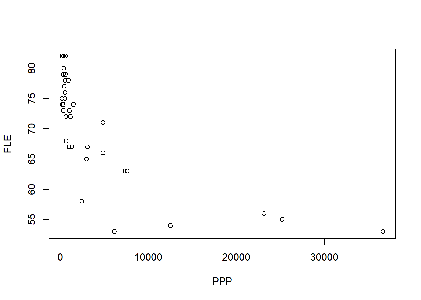
Figure 5.1: Scatterplot of female life expectancy versus the number of people per physician.
As the relationship appears to be non-linear, we apply log-transformation to the predictor variable. Transforming the values of \(x\) might be the first thing to try if there is a non-linear monotonic (i.e. entirely non-increasing or entirely non-decreasing) trend in the data, and non-linearity is the only problem. In other words, model assumptions (i.e. independence, zero-mean, constant variance, normality) should be met. The scatterplot of female life expectancy against \(\log\)(PPP) is produced using:
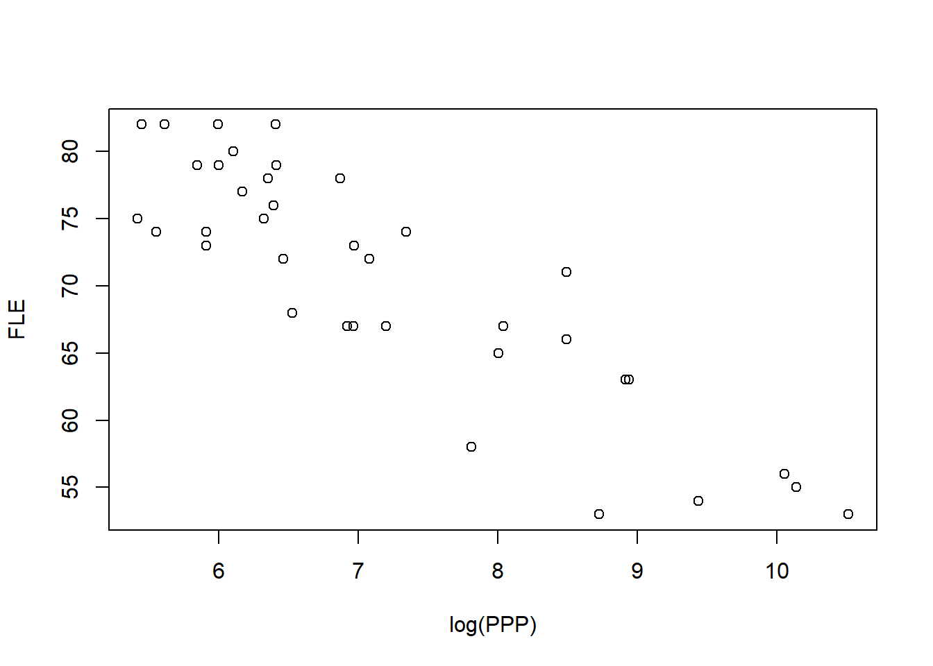
Figure 5.2: Scatterplot of female life expectancy versus log(number of people per physician).
Figure 5.2 shows a linear trend after transforming \(x\). Therefore, we will model the relationship between FLE and \(\log\)(PPP) using a simple linear regression model. The model is given as: \[Y_i = \beta_0 + \beta_1 \log(x_i) + \epsilon_i,\quad \epsilon_i \sim N(0,\sigma^2), \quad i = 1,\ldots, 37.\]
5.1 Statistical analysis
A simple linear regression model can be fitted by using the lm command:
The summary table and ANOVA table of this model can be produced by using summary() and anova():
##
## Call:
## lm(formula = FLE ~ log(PPP), data = life)
##
## Residuals:
##    Min     1Q Median     3Q    Max
## -9.065 -3.489  1.143  2.663  7.674
##
## Coefficients:
##             Estimate Std. Error t value Pr(>|t|)
## (Intercept) 109.9498     3.6860   29.83  < 2e-16 ***
## log(PPP)     -5.4893     0.5036  -10.90 8.48e-13 ***
## ---
## Signif. codes:  0 '***' 0.001 '**' 0.01 '*' 0.05 '.' 0.1 ' ' 1
##
## Residual standard error: 4.286 on 35 degrees of freedom
## Multiple R-squared:  0.7724, Adjusted R-squared:  0.7659
## F-statistic: 118.8 on 1 and 35 DF, p-value: 8.484e-13## Analysis of Variance Table
##
## Response: FLE
## Df Sum Sq Mean Sq F value Pr(>F)
## log(PPP) 1 2182.34 2182.34 118.81 8.484e-13 ***
## Residuals 35 642.91 18.37
## ---
## Signif. codes: 0 '***' 0.001 '**' 0.01 '*' 0.05 '.' 0.1 ' ' 15.2 Assumption checking
As seen in previous examples and exercises, model assumptions can be assessed graphically by producing a plot of the residuals versus the fitted values and a normal probability plot (Q-Q plot) of the residuals. It is important to check the assumptions of your model are met before using it.
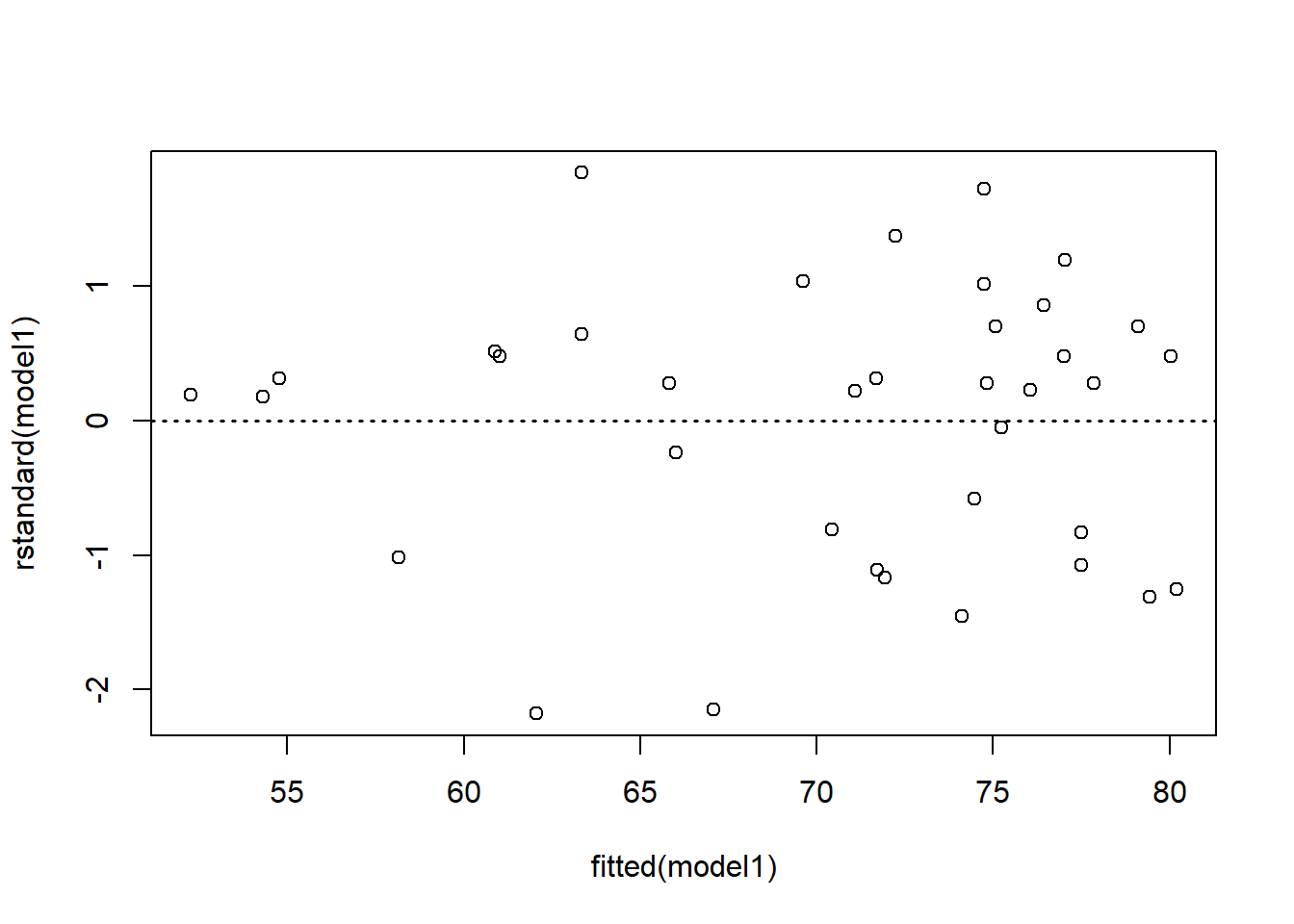
Figure 5.3: Standardised residuals versus fitted values plot from fitting a simple linear regression model to transformed variables.
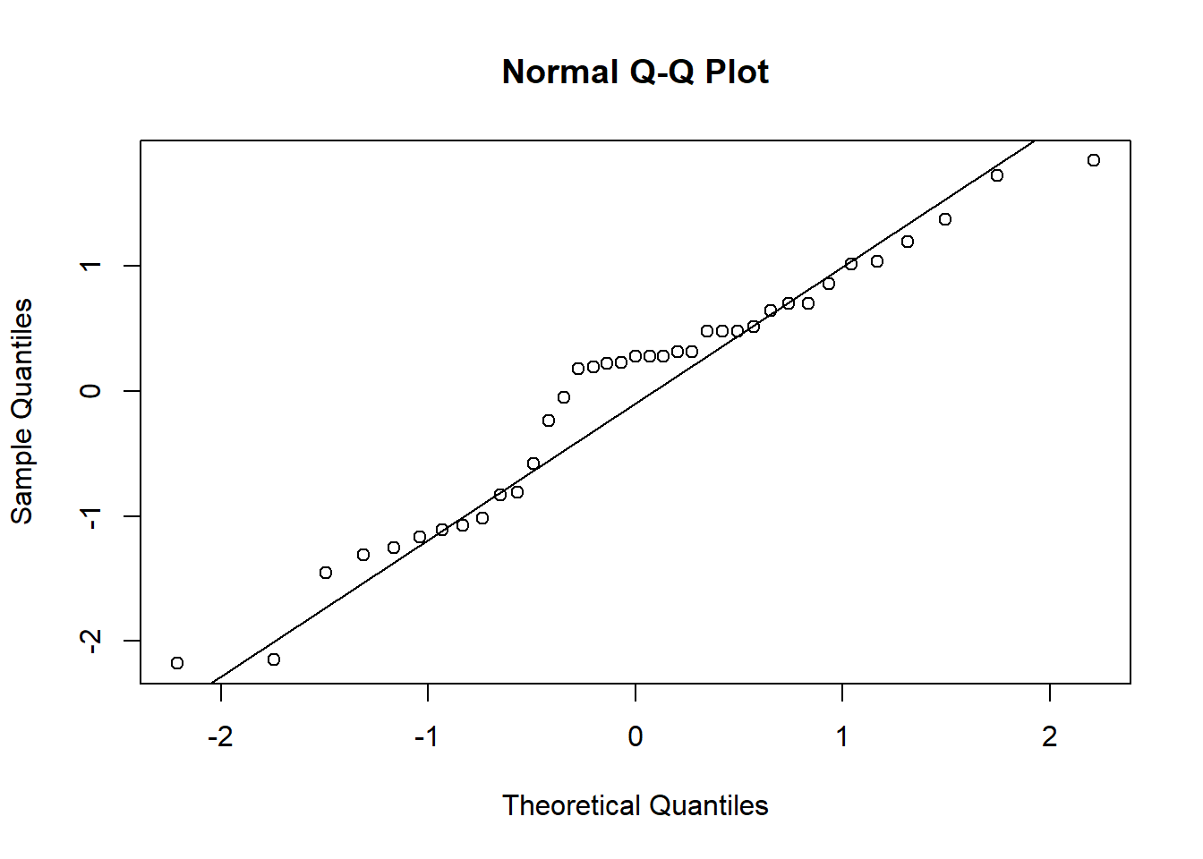
Figure 5.4: Normal probability (Q-Q) plot from fitting a simple linear regression model to transformed variables.
Figure 5.3 displays the residual plots after fitting a simple linear regression model to the transformed variables. The points are fairly evenly scattered above and below the zero line, which suggests it is reasonable to assume that the random errors have mean zero. The vertical variation of the points seems to be small for small fitted values. However, there are also less points in this case. It would be preferable if more data are available. In the normal probability plot (Figure 5.4), we see that points do not exactly lie on diagonal line. This indicates that the normality assumption may not necessarily be satisfied. The independence of the random errors seems to be reasonable since each point refers to a different country.
QUESTIONS:
- Using the following summary statistics, calculate the least squares estimates of \(\beta_0\) and \(\beta_1\). Check your answers with the column of
Estimatein the summary table.
\[\bar{x} = 7.18,\ \bar{y} = 70.51,\ S_{xx}=72.42,\ S_{yy}=2825.24,\ S_{xy}=-397.56\]
\[\hat{\beta_0} = \bar{y} - \hat{\beta_1}\bar{x},\ \hat{\beta_1} = \frac{S_{xy}}{S_{xx}}\]
- Write down the equation of the fitted model. Based on it, comment on the least squares estimate of \(\beta_1\) and predict the value of female life expectancy when the number of people per physician equals 4000.
The regression equation is \[\text{FLE} = 109.95 - 5.49 \cdot \log(\text{PPP})\]
\(\hat{\beta_1}\) can be interpreted as: if \(\log(\text{PPP})\) increases by 1 unit, the expected female life expectancy decreases by 5.49.
When predicting the value of the response for a new observation, we need to back transform the variable. For example, if the number of people per physician is 4000, the best prediction of female life expectancy is \(109.95 - 5.49 \cdot \log(4000) \approx 64.42\).
- Use the summary statistics in (a) to complete the analysis of variance table below, i.e. finding the degrees of freedom, the sum of squares, the mean squared error, and the \(F\)-statistic. Check your answer with the
anovaoutput.
| Component | DF | Sum Sq (SS) | Mean Sq (MS) | F |
|---|---|---|---|---|
| Model | ||||
| Residual | ||||
| Total |
- What hypotheses are being examined by the \(F\)-statistic in the ANOVA table? By looking at its \(p\)-value, what can you conclude about the fitted model?
The null and alternative hypotheses are: H\(_0\): \(\beta_1=0\) versus H\(_1\): \(\beta_1 \neq 0\). Note that \(\beta_0\) is not included in the hypothesis.
Since the \(p\)-value (from Pr(>F)) is less than 0.05, we reject the null hypothesis and conclude that \(\log\)(PPP) is useful in predicting FLE.
- Compute and interpret the coefficient of determination, \(R^2\). Check your answer with the term
Multiple R-squaredin the summary table.
\[R^2 = 1-\frac{SSE}{SST}\]
\[\begin{equation*} \begin{split} R^2 &= 1-\frac{SSE}{SST}\\ &=1-\frac{642.91}{2182.34+642.91}\\ &=0.772 \end{split} \end{equation*}\] The \(R^2\) tells us the model provides a relatively adequate fit to the data with 77% of variability in FLE can be explained by this model.