Lab 10 - Transformations and Assumptions
1 Welcome to Lab 10!
Intended Learning Outcomes:
- Produce residual plots and assess the assumptions of a linear model.
- Fit linear models with transformed variables.
1.1 Introduction to variable transformations
The need to transform variables may arise during the exploratory analysis when you realise that your predictor(s) do not have a linear relationship with the response, or during assumption checking when the residuals do not meet assumptions. In either case, a transformation of the response variable, the predictors, or both response and predictors may be necessary.
If the model has been fitted using a transformation on the response variable, the results will be given in the transformed scale. It is still possible to report the findings in the original scale, but this requires a back-transformation. How do I back-transform my data, you ask? Simply apply the inverse operation (inverse of the transformation) to your predictions.
In this lab, we will explore some simple transformations and how to tell if you need them. All examples are a simple linear regression where \(Y = \beta_0 + \beta_1 x + \epsilon\), where \(Y\) is the response and \(x\) is the predictor.
1.2 Root
A root transformation is one where you take a root of the variable. For example, you may take the square or cubic root. Recognising the need for the transformation is important. Here is a small simulation to give you a taste for a predictor in need of a square root transformation looks like. In this example, \(\beta_0 = 1\) and \(\beta_1 = 2\).
par(mfrow = c(1,2))
plot(Y~x, pch = 16,
     main = "Original Scale")
plot(Y~I(x^0.5), pch = 16,
    main = "After Square-root Transformation")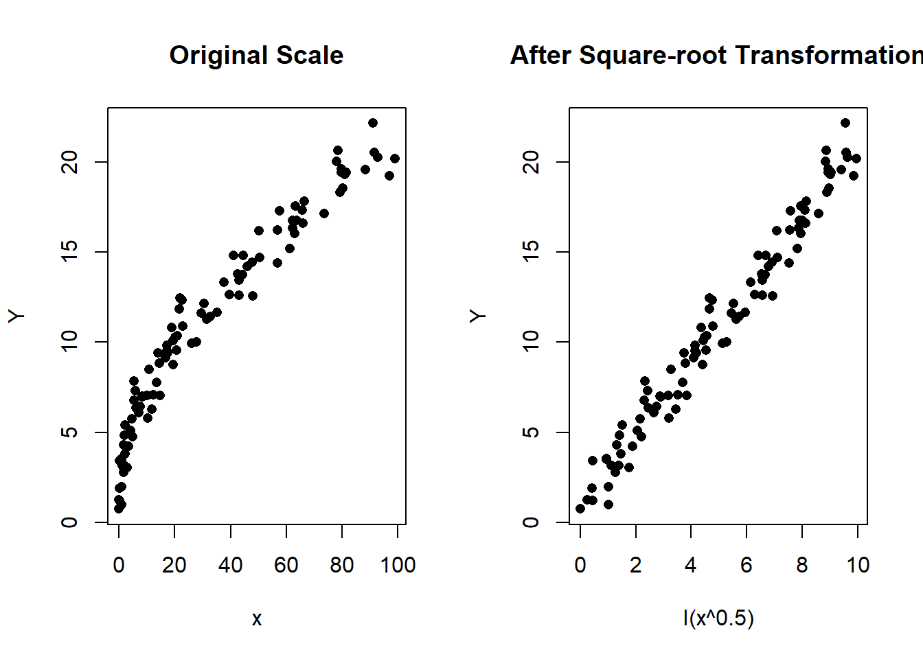
Figure 1.1: Left: Scatterplot of Y vs x in the original scale. Right: Scatterplot after the square-root transformation of \(x\)
As you can see in the plots, the transformation may be required if the predictor displays a convex curved relationship with the response. If you think this is you, you can apply the transformation in the model using:
1.3 Reciprocal
The reciprocal transformation of \(x\) is the same as saying \(\frac{1}{x}\) or \(x^{-1}\). We performed another simulation to show you what data in need of the reciprocal transformation look like. Here, \(\beta_0 = 1\) and \(\beta_1 = 1.5\).
par(mfrow = c(1,2))
plot(Y~x, pch = 16,
     main = "Original Scale")
plot(Y~I(x^-1), pch = 16,
    main = "After Reciprocal Transformation")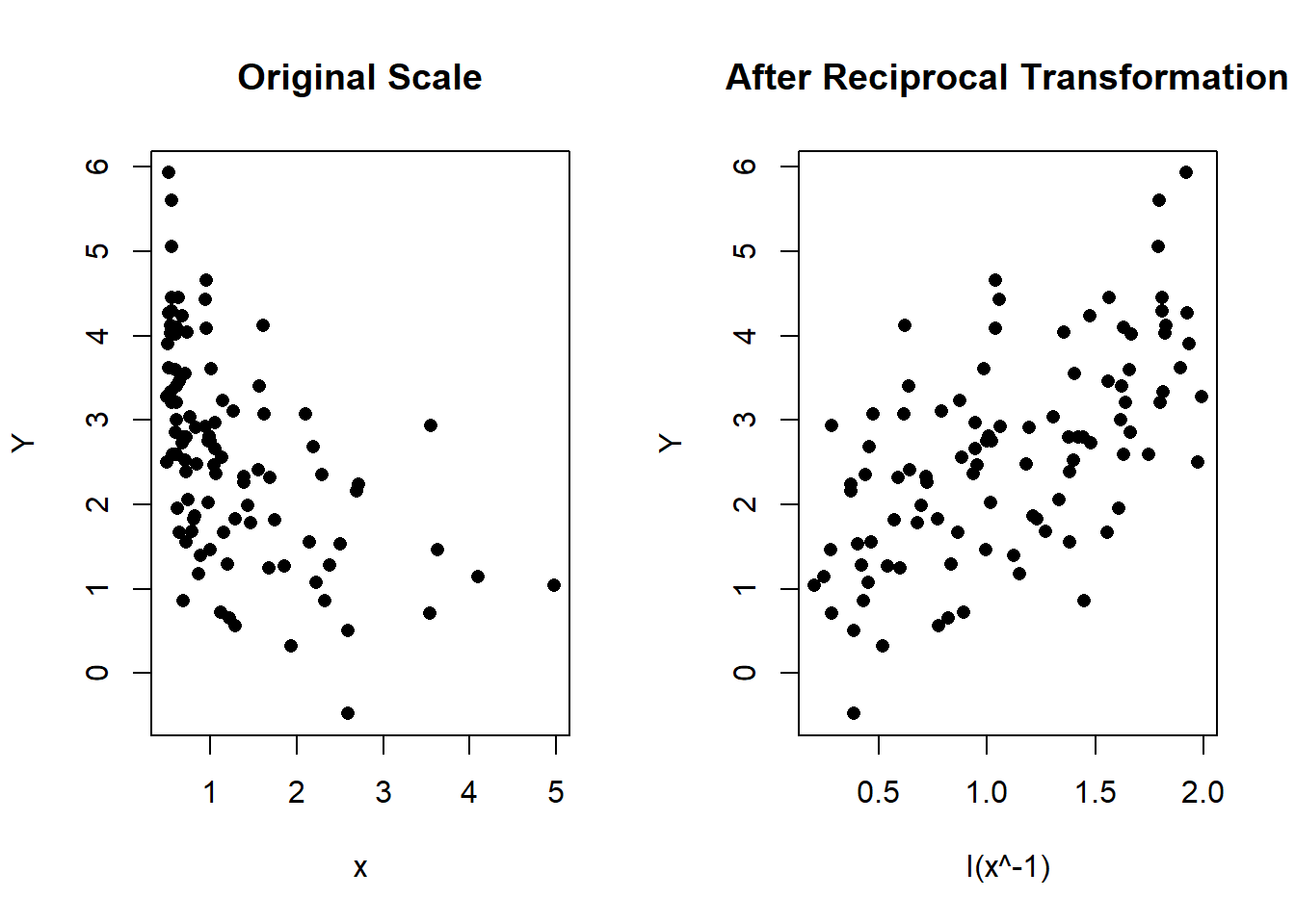
Figure 1.2: Left: Scatterplot of Y vs x in the original scale. Right: Scatterplot after the reciprocal transformation of \(x\)
The figure shows a concave curve that slopes downward. The response is largest when \(x \leq 1\) because \(\frac{1}{x} > 1\) when \(x < 1\). Using the same logic, we understand that large values of \(x\) result in smaller values of \(Y\).
You can fit it in a model using:
1.4 Quadratic
The quadratic transformation of \(x\) is the same as saying \(x^2\). It is the inverse of the square-root transformation. It it a subset of the power transformations. In more general terms, it is \(x^a\), where \(a\) is anything. The reciprocal can also be thought of in this same category.
But what does it look like? The figures below are a simulated example using \(\beta_0=1\) and \(\beta_1=2\).
par(mfrow = c(1,2))
plot(Y~x, pch = 16,
     main = "Original Scale")
plot(Y~I(x^2), pch = 16,
    main = "After Quadratic Transformation")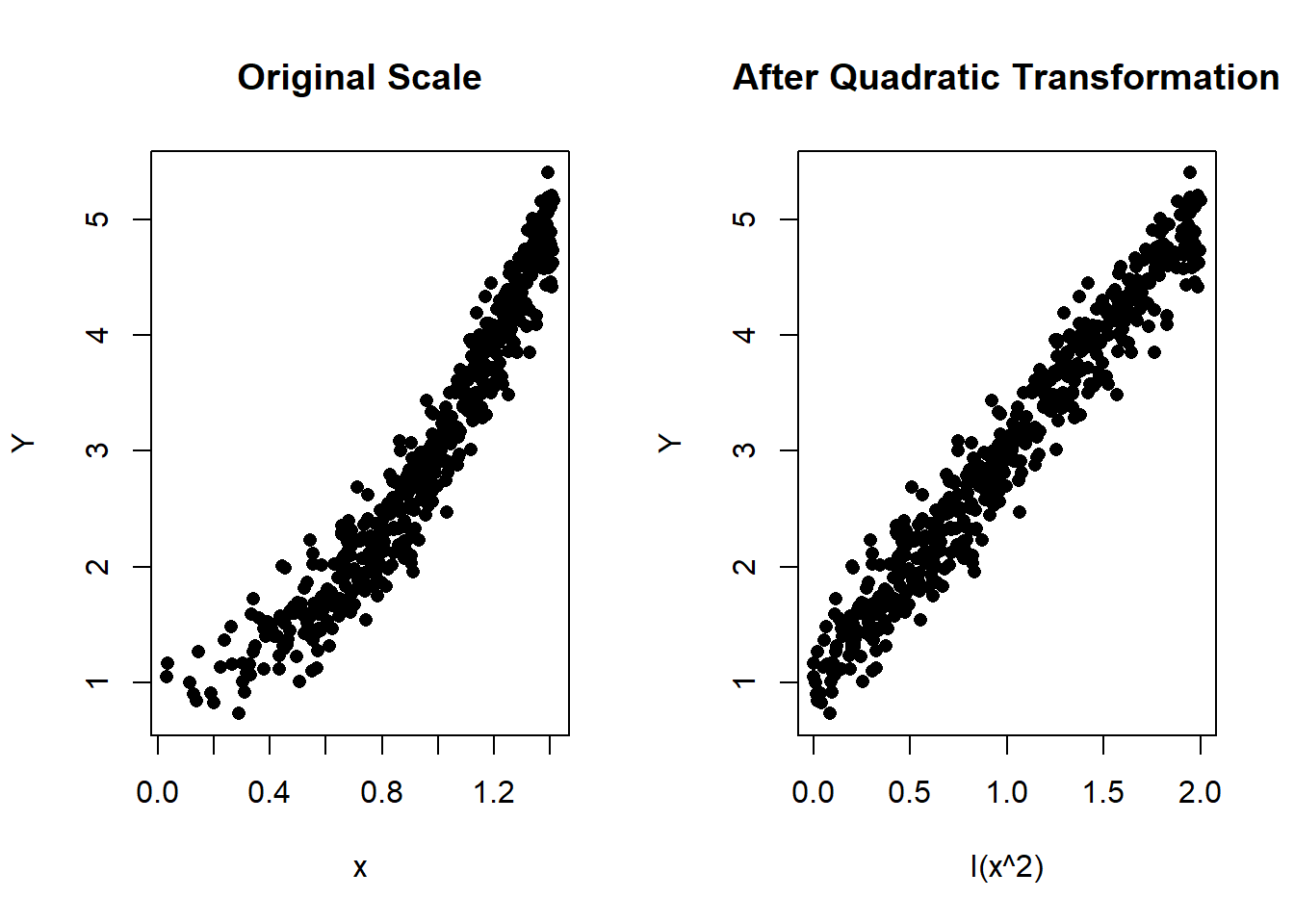
Figure 1.3: Left: Scatterplot of Y vs x in the original scale. Right: Scatterplot after the quadratic transformation of \(x\)
As you can see from the plots, the predictor has a concave relationship with the response previous to the quadratic transformation. You can use it in a model by using the code:
1.5 Logarithmic
Last but not least, the logarithmic transformation is equivalent to saying \(\ln(x)\), which in R is the same as log(x). Here is another simulation that shows the original and transformed predictor when the transformation should be logarithmic.
par(mfrow = c(1,2))
plot(Y~x, pch = 16,
     main = "Original Scale")
plot(Y~log(x), pch = 16,
    main = "After Log Transformation")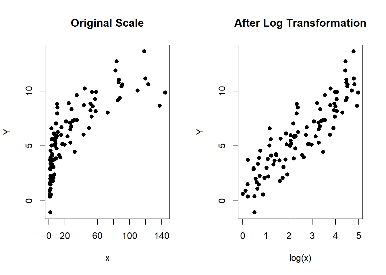
Figure 1.4: Left: Scatterplot of Y vs x in the original scale. Right: Scatterplot after the log transformation of \(x\)
Fitting the transformation in R is straight forward as in the previous transformations. You can use:
# Model without transformation
model <- lm(y ~ x)
# Model with transformation
model.root <- lm(y ~ log(x))
Another useful feature of the logarithmic transformation is that it can help when applied to the response variable too so that both predictor and response are log-transformed. In the original scale, the data can look like this:
par(mfrow = c(1,2))
plot(Y~x, pch = 16,
     main = "Original Scale")
plot(log(Y)~log(x), pch = 16,
    main = "After Log Transformation")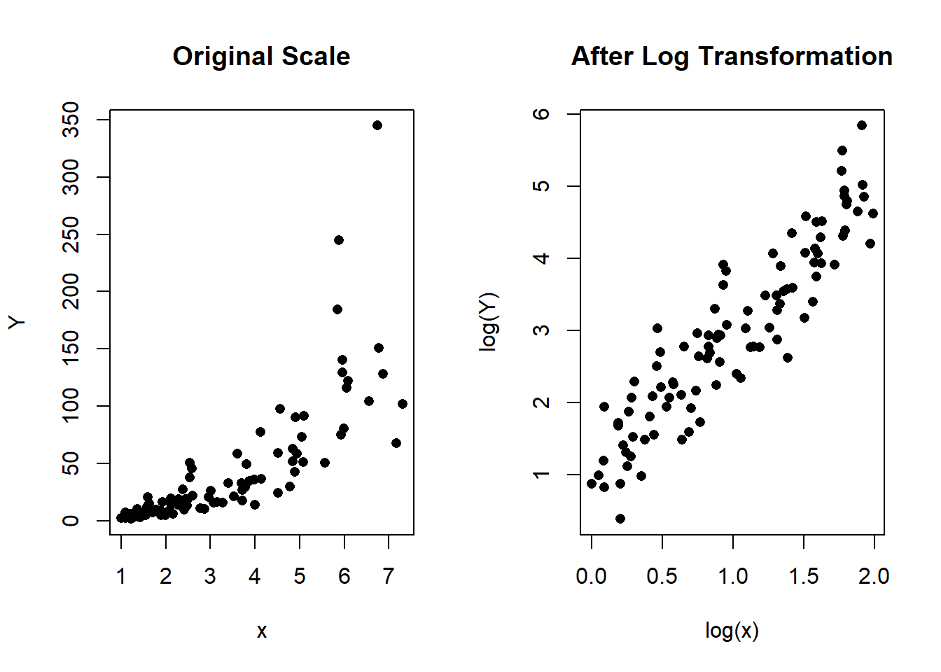
Figure 1.5: Left: Scatterplot of Y vs x in the original scale. Right: Scatterplot after the log transformation of \(x\) and \(Y\)
The main thing to note in these plots is the increasing variance the further away from the origin. Sort of like a "fanning" effect. The transformation is easy to fit using:
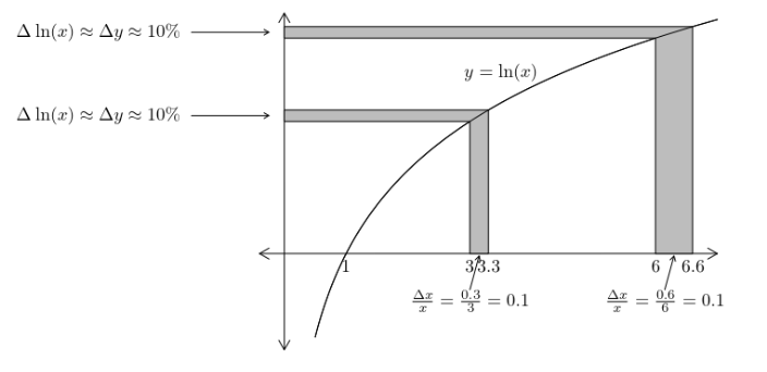
You will not need to know this for the exam, but as a special feature, models that use logarithmic transformations have approximate interpretations without the need for back-transformation. When \(x\) has been transformed with a natural log transformation, the change in the \(\ln(x)\) is roughly equal to the change in \(x\) provided the changes in \(x\) are small. Consider the figure below, which graphically illustrates how changing the \(x\) values 3 and 6 by 10% corresponds to an approximate increase in \(\ln(x)\) of about 10%.