3 Example 2: Animal brains and double transformations
Variables are often transformed to fix constant variance or normality assumptions; however, transformations can complicate the interpretation of the model. In this example, we explore transforming both the response and the predictor(s). To illustrate what we mean, we will use the data frame Animals from the MASS package. The data consists of 28 animals, including dinosaurs, and their respective body weight in kilograms and brain weight in grams. Our question of interest is: is a bigger brain required to govern a bigger body?
Data: Animals
Columns:
body - body weight given in kilogramsbrain - weight of brains given in gramsRead the data using:
Exploratory analysis and model fitting As always, it is important to first plot the data to understand the relationship between response and predictor in the original scale. Before you start, make sure to remove the dinosaurs from the data (observations 26 to 28 after sorting), because they are outliers (which we know from previous labs!).
# Sort by body size
SA <- Animals[order(Animals$body), ]
# Remove dinos
NoDINO <- SA[-c(26:28),]
# Plot the data
plot(NoDINO, pch = 16, xlab = "Body", ylab = "Brain")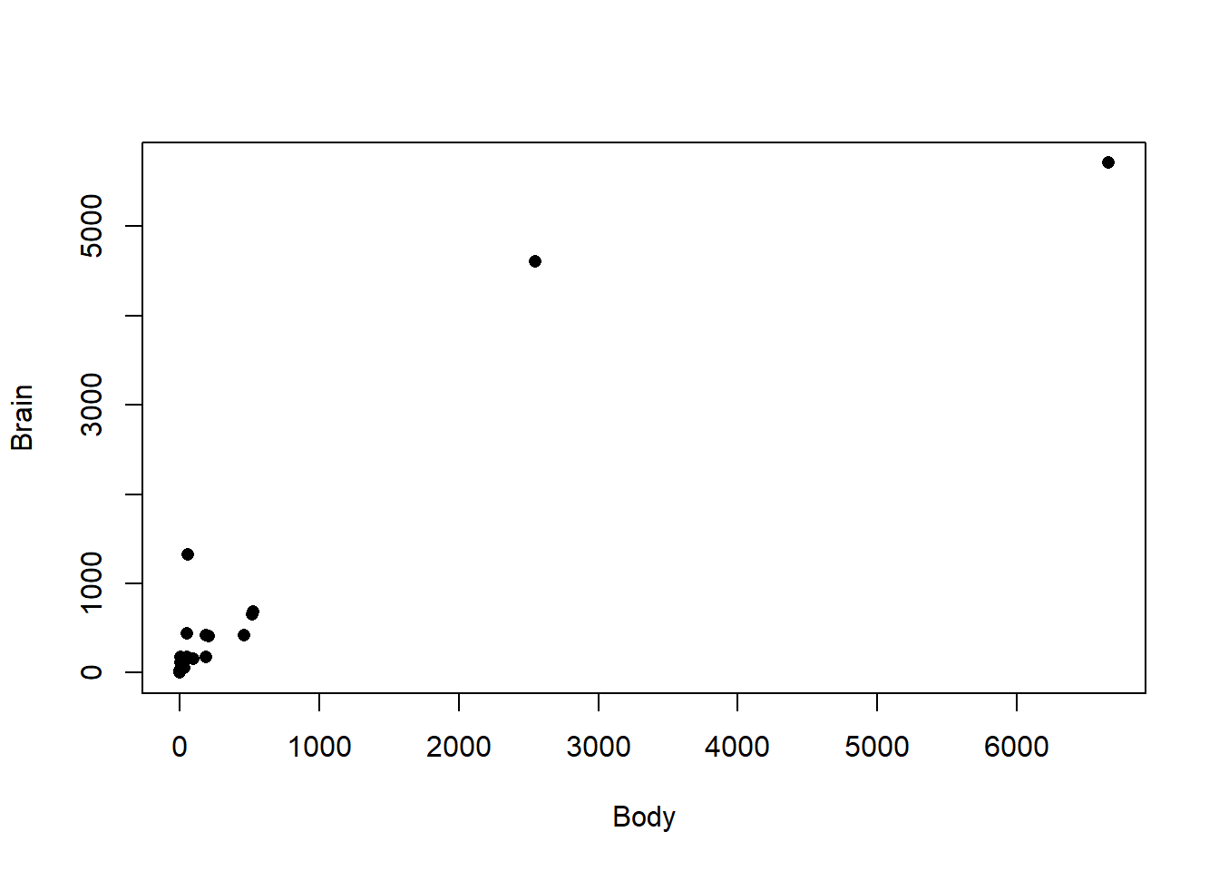
From the figure above, we can see the response and predictor have a difficult relationship that is curved (convex) and increases in variability. Transforming both variables may be useful in this case. From the introduction, we know logarithmic transformations are often a good choice.
You can fit this model in the same way that you have fitted the other transformations.
## (Intercept) log(body)
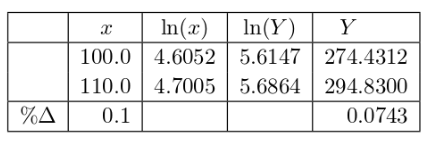
## 2.1504121 0.7522607Interpretation The predicted log(brain weight) of the jaguar, whose body weight is listed as \(100 \text{kg}\) with the fitted model, is \(2.1504+0.7523\times\text{ln}(100)=5.6147\). This must be back transformed to get the units of original brain measurement (grams). The brain weight predicted by the model is \(\exp(5.6147) = 274.4312 \text{g}\).
When both the response and the predictors have been transformed with a natural logarithm, one can use the percentage interpretation of \(\beta_1\) and be very close to the actual change given by the model for small changes in the \(x\)-variable. If the body weight of an animal increases by \(1\%\), the approximate increase in brain weight is \((0.01\times0.7523 = 0.007523 = 0.7523\%)\) since \(\hat{\beta}_1= 0.7523\). If the jaguar were to increase its weight by \(10\%\), the expected increase in brain weight would be approximately \(7.5\%\) for a new weight of \(1.075 \times 274.4312 = 295.0136 \text{g}\). The actual brain weight change predicted by the model for a body weight of \(110 \text{kg}\) is \(294.83 \text{g}\) and the change in brain weight as predicted from the model is \(7.4331\%\) (see Table 1). Note that for this model, \(\hat{\beta}_1= 0.7523 \approx \% \Delta Y /\% \Delta x = 0.0743/0.1 = 0.7433\). In fact,